Assignment 3-2D Element Formulation Challenge
2D BAR SIMULATION AND COMPARISON WITH DIFFERENT PROPERTY CARDS
PROCEDURE
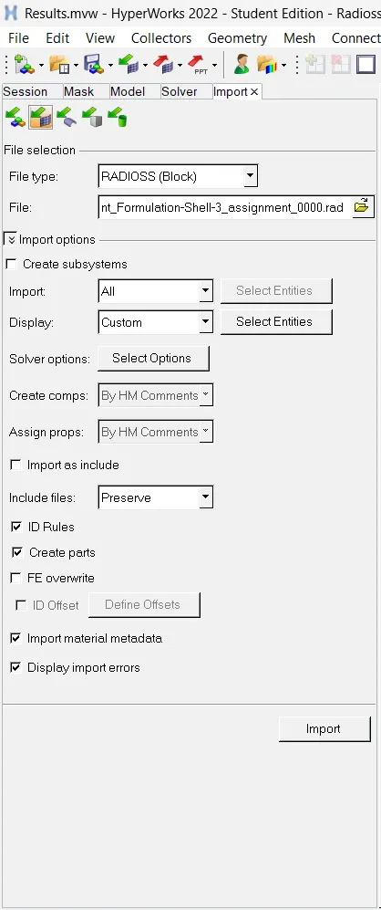
1. We shall be changing a couple of simulation properties by accessing them through Hyperworks. This first question requires us to change the run time to 55 ms. For that, we first need to import the solver deck file in question to RADIOSS.
For that, we need to go to File > Import > Solver Deck. This brings up the import menu. Here, we can select the file we need to import. The file would be the starter input deck file (which is the file that ends with '0000.rad').
With the model imported, we can go ahead and change the run time to 55 ms (as required). To do that, we need to proceed to the solver tab in the sidebar. Proceeding to ENGINE_KEYWORDS > RUN > ENG_RUN, we can now edit properties of ENG_RUN in the small window below the tab.
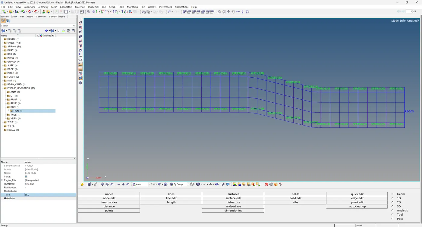
Here, we can change the Tstop">Tstop����� value to 55.
2. The next question requires us to change the number of simulation steps to a minimum of 25 and a maximum of 60. For this, we need to go to the same solver tab and proceed to ENGINE_KEYWORDS > RUN > ANIM > ANIM/DT. We shall be changing this particular attribute's properties.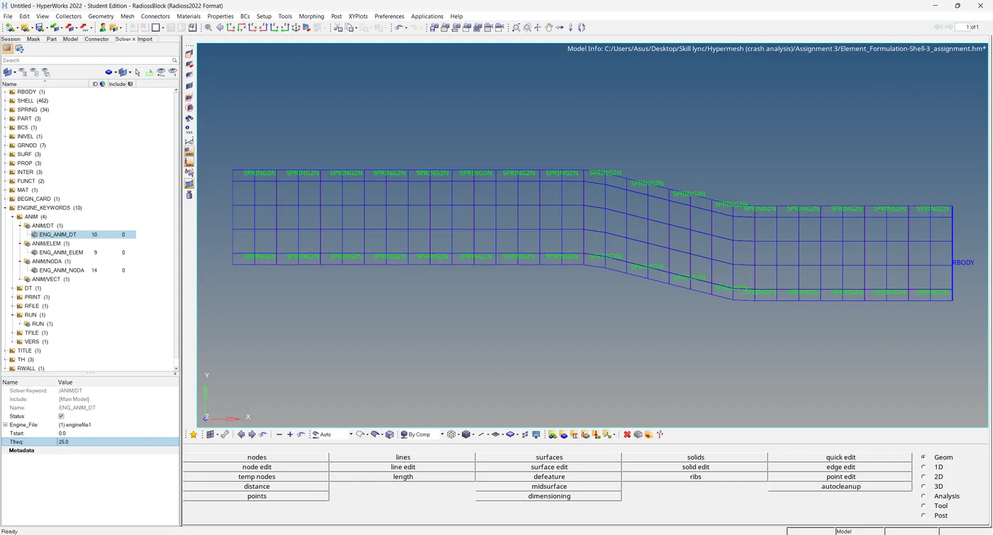
In the property section, we can change the Tstart">Tstart������ value to 25 and to accommodate a maximum of 60 animation steps, Tfreq">Tfreq����� can be set at 1.
3. Next requirement is to run the base simulation. For that, we need to save the current file with edited parameters. This can be carried out via the analysis process.
For this, we can go to the 'Analysis' section from the bottom panel.
There, we can select RADIOSS.
In the next section, we are given the option to save the file before running it in the solver. We can go ahead and give it a different name from the base file to avoid confusion. Clicking 'save as' lets us do that.
After saving, before running it into the solver, we can activate 'include connectors' and in the options bar, we need to enter "-nt 4" to increase the processing power of the solver (as in to use all 4 cores). After that, we can click 'Radioss' to activate the solver and it processes t the file. We get a solver window that tells us what's going on in the process. It runs for several seconds before finishing and letting us know about completion.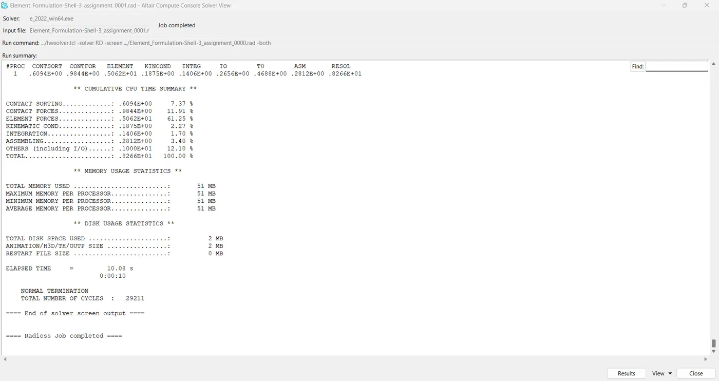
The simulation is complete, now we just need to visualize it. For that, we need to switch to the Hyperview utility. This can be done by clicking the client selector option in the toolbar (might need to be activated from View > Toolbars > Hyperworks > Client Selector). In that menu, we can select Hyperview to switch to it.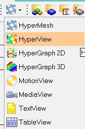
After accessing Hyperview, we are asked to input the simulation file. For this, we shall be using the h3d file that was generated when RADIOSS processed the starter file. It should be generated in the same folder. After selecting it, we can click 'apply'.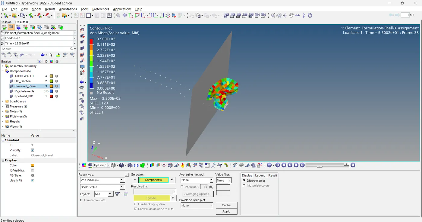
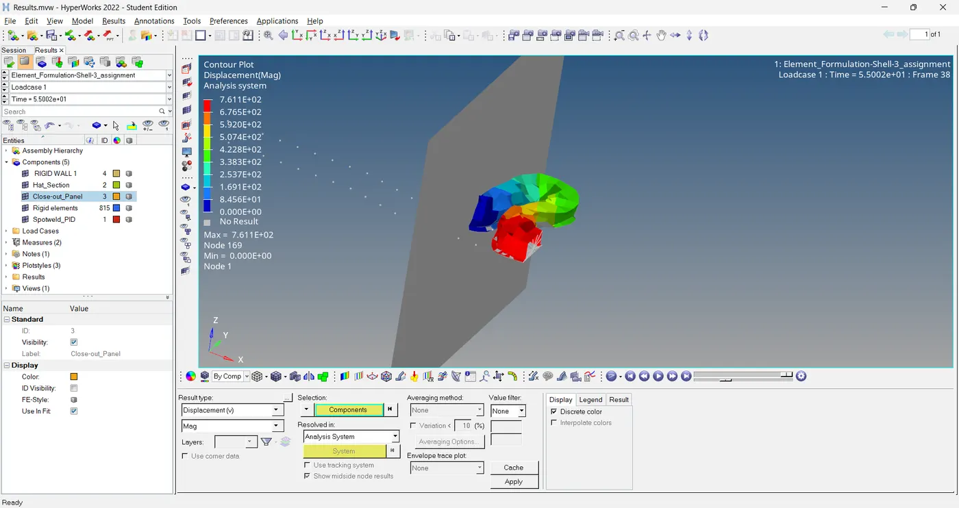
Doing so generates the simulation animation. We can change what is being represented by selecting the 'contour' option in the toolbar.
The following simulation depicts displacement:
The following animation depicts Von Mises stress in the component during the simulation:
4. Next step is to carry out energy error and mass error checks and this is done by analyzing the RADIOSS engine output file. This can be accessed from the same directory as the starter and engine files and is denoted by the '.out' extension. We need to check the file that contains '_0001.out' by using any text editor.
On opening the file and scrolling down to the end, we can see the final energy and mass error values.
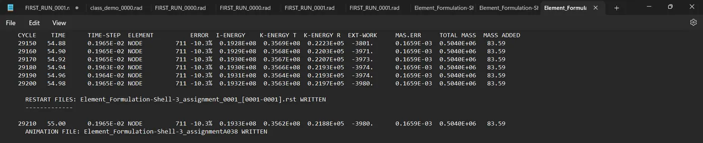
The final energy error is -10.3%, which is less than the threshold of -15% and is acceptable. Acceptable energy error values are supposed to be between -15% and 10%. The closer to 0 it is, the better.
5. With the energy and mass errors deemed acceptable, we can go ahead and plot the graphs. For this, we shall be using the Hypergraph client. We can switch to it using the same client selector option in the toolbar.
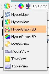
In the Hypergraph section, we are met with a graph and in the panel below, we are to input a file. For this, we will be using the result file generated by the RADIOSS solver (also known as the 'T01 file'). This file is available in the same directory as the starter, engine and animation files. The file name ends with 'T01'.
After adding it, we can select the variables that would go with time (x axis).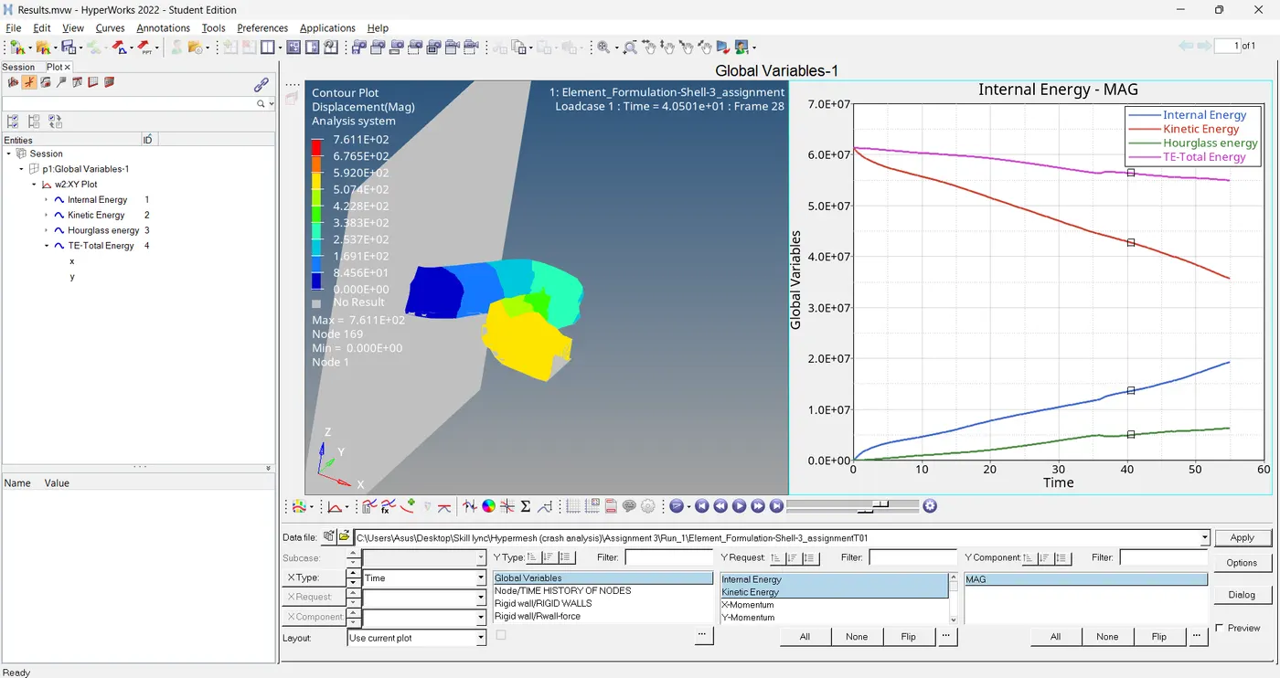
First, we can take a look at the energy graphs (internal energy, hourglass energy, contact energy, kinetic energy and total energy)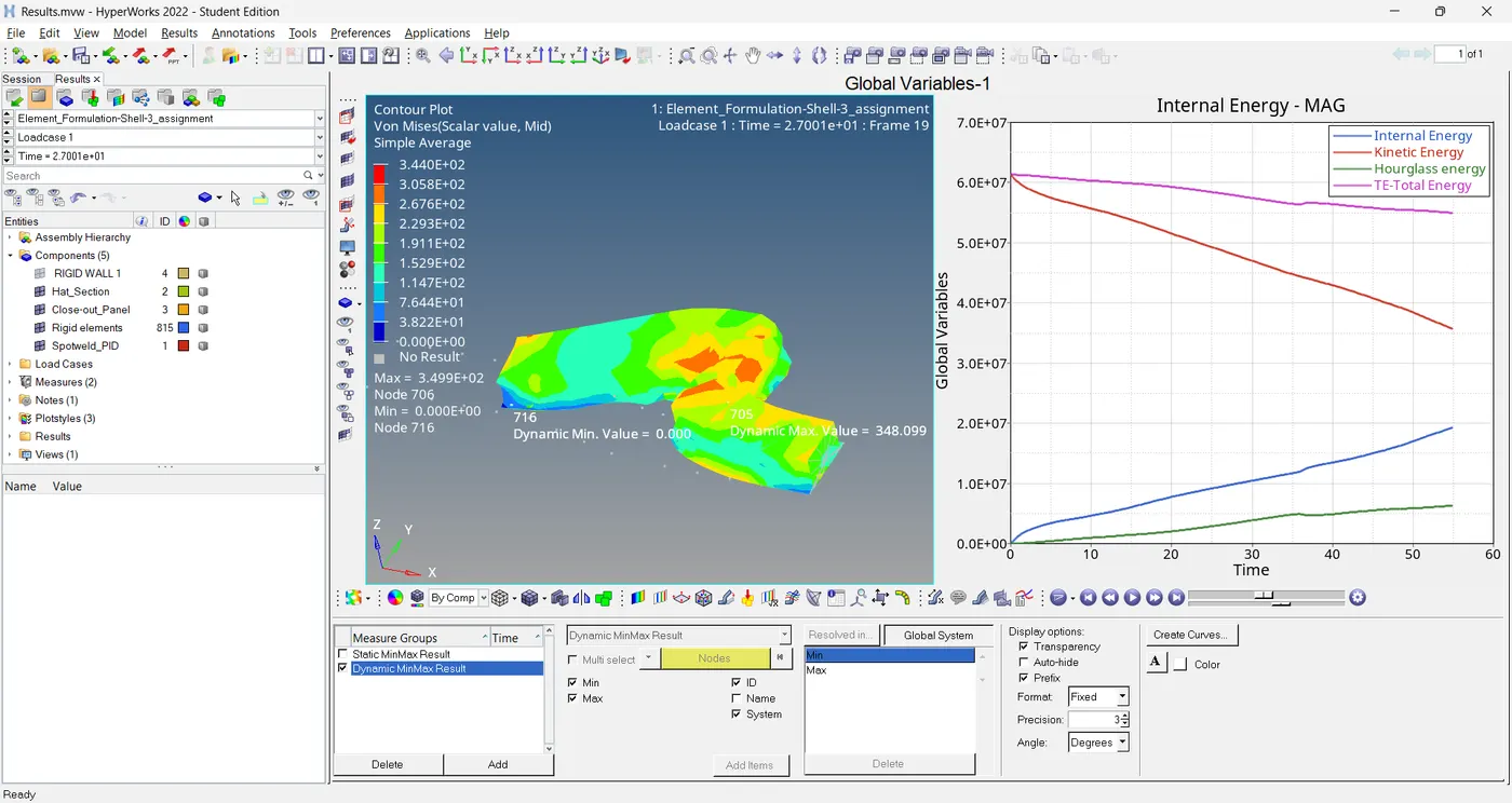
Now to generate the graph for rigid wall forces (Rigid Wall/Rwall Force - 4 RIGID WALL 1 - total resultant force).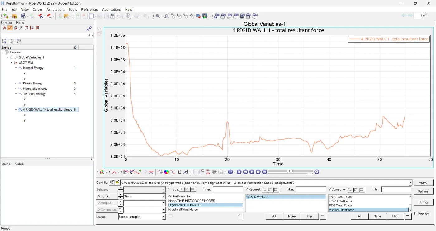
6. For this question, we are to carry out a simulation for a new case with the recommended shell element properties. We can repeat the process of importing the original solver deck file and change the values of Tstop">Tstop����� , Tstart">Tstart������ & Tfreq">Tfreq����� in the solver tab.
After that, we can move to the model tab and go to the properties submenu. The shell properties of the model's components are to be changed so we need to select each of 'Hat-Section' and 'Close-Out Panel' one-by-one and change the values in the property window below as shown:
As specified, Ishell">Ishell��ℎ��� would be 24, Ismstr">Ismstr������ would be 2, Ish3n">Ish3n��ℎ3� would be 2, N would be 5, Ithick">Ithick��ℎ��� would be 1 and Iplas">Iplas����� would be 1. These values are changed for both aforementioned components.
After they're changed, we need to generate the RADIOSS analysis file again via Analysis > RADIOSS in the bottom panel. We can save it in a different name and assign the same settings as the previous case (option: "-nt 4" and with 'include connectors' checked. The solver file is then generated by clicking Radioss.
After that, we can switch to Hyperview to generate the simulation. Like last time, we need to pick the h3d file of this case and click apply.
The following animation shows the Von Mises stress contours for the component using recommended shell formulation settings:
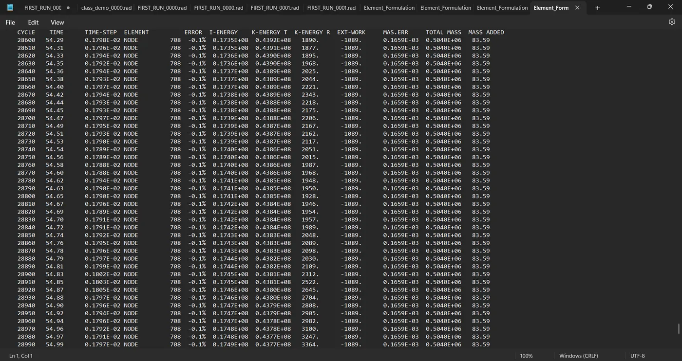
7. Having generated the simulation, we can go ahead and carry out energy and mass error checks, again using this particular simulation's RADIOSS output file. This can be accessed from the same directory as the starter and engine files of this simulation and is denoted by the '.out' extension. We need to check the file that contains '_0001.out' by using any text editor.
As we can see, there is a drastic reduction in energy error, as was evident in the more natural-looking simulation (reduction in hourglass energy).
Now we can generate the graphs by switching to Hypergraph and selecting this simulation's T01 file. Firstly, the energy graph: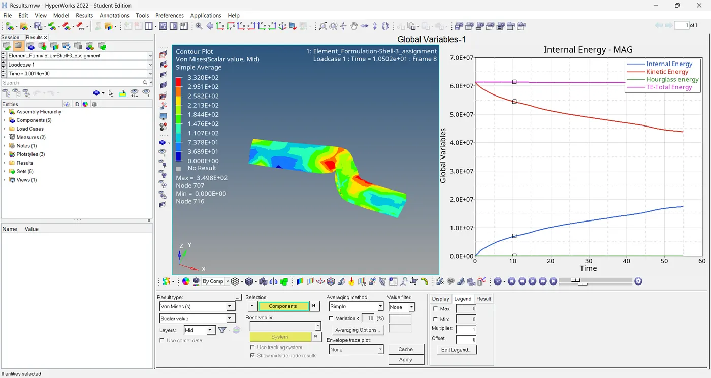
As we can see, there is almost no hourglass energy and this corresponds with the energy error observation.
Now we shall generate the graph for rigid wall forces:
8. & 9. The obvious difference in both simulations is the reduction in hourglass energy. The introduction of QEPH shell formulation (Ishell">Ishell��ℎ��� = 24) in the second case, provides an artificial stiffness to the shell elements and helps counter hourglass formation.
A result of hourglass reduction is the more 'natural' looking simulation in the second case, with less crumpling.
A reduction in hourglass means a reduction in hourglass energy since an artificial, external force needn't be applied to negate the hourglass formation (as in the case of Q4 elements).
This, in turn, affects the total energy in the system. When recommended settings are applied, with no loss of energy to hourglass energy, the total energy in the system is maintained.
The more realistic simulation also resulted in a different resultant force graph that represents the collision events more realistically. The formation of a kink at around 20 ms causes a sudden spike in case 1, whereas in the second simulation, as the QEPH shell formulation is used, there is no sudden spike as the elements are deformed in a much better manner. Understandably, there is a large force at the beginning, which happens at contact, and is the same in both cases.
Overall, there have been some obvious differences in results. To summarize:
| Attribute | Simulation with Default properties | Simulation with recommended properties |
| Energy Error | -10.3% which is acceptable (average result) | -0.1% A good number since it's almost 0. |
| Total energy | Total energy reduces over time due to the introduction of hourglass energy | Total energy remains constant since there is barely any hourglass energy |
| Hourglass Energy | Hourglass Energy increases over time | Hourglass energy remains zero |
RESULTS
Two simulations were carried out on the same crush beam using different shell element formulation properties.
Comparing the results of both cases, it can easily be figured out that there is a big difference in the values of hourglass energy, internal energy, kinetic energy, total energy and rigid wall forces.
Also, the amount and nature of deformation of the 2nd case are much higher and different than the first case. This deformation is more practical than the base simulation. This improvement is definitely due to changes in the material card and its element properties which resulted in the reduction of hourglass energy.
It was established that using the recommended settings helped reduced hourglass formation drastically due to the introduction of the physical stabilization method that is deployed by QEPH elements.
REFERENCE LINKS
https://drive.google.com/file/d/1DPAGvCKuCkJND0Y8OZ67Wow-gryl55GG/view?usp=sharing
https://drive.google.com/file/d/1lbM3gLuNFR-mzvje0ORizhVk0ECbHDTa/view?usp=sharing
https://drive.google.com/file/d/1NqDG2xOwgy99_z-LI9nfodSj8G2-sOQB/view?usp=sharing
https://drive.google.com/file/d/1K0USOMDtmDhPSYipaRXYq2eswpXwXTj6/view?usp=sharing
https://drive.google.com/file/d/1oQH5Wb06XLG13mDeIqnyHVG7fu7u9F43/view?usp=sharing