Assignment 3-2D Element Formulation Challenge

1.Using the crash beam file from the previous assignment, change the run time to 55 ms.
Ans: Import solver-deck file. Go to 'cards' in browser. Select 'ENG-RUN' card. Edit T-stop value as 55 in entity editor.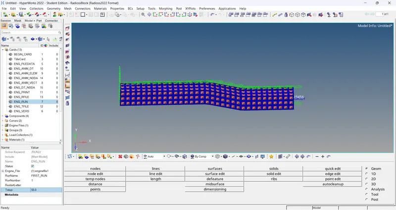

2.Change the number of animation steps during simulation to a minimum of 25 and maximum of 60.
Ans: Assume number of animation steps are '55'. Select 'ENG_ANIM_DT' card. Edit Tfreq value as '1' in entity editior.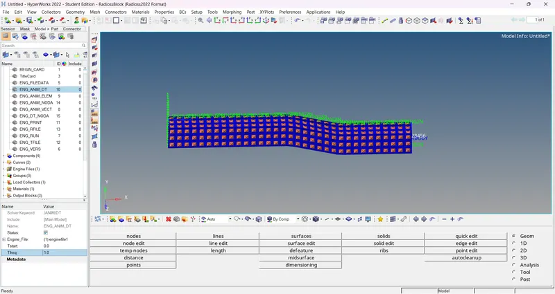

Objectives: To run the simulation with base setup and with improved shell elements properties and comapare the results between them.

Procedure:-

Case 1: Base Simulation

1. Import the solver deck and import the starter(0000.rad) file.
2. To run simulation, Go to 'Analysis' panel and select 'Radioss' option. Ensure the input file and select 'export option' and 'run option' as 'all' and 'analysis' resp. Then enter '-nt 4' in options and click on 'radioss'.
3. After click on radioss, 'compute console solver view' window is open. Then check the energy error and click on 'Results'. And the hyperview window is opened. Select '.h3d' file in 'load model' and 'load result' option and click on apply.
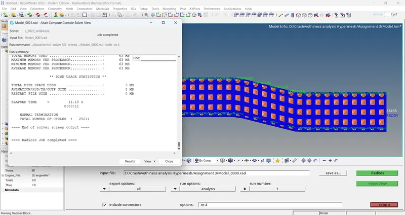
4. Then enable shaded elements and mesh lines. After that click on contour and select result type as 'Von Mises(s)' and hit on apply. Then click on page window layout and select 'split the window in 2 parts'.
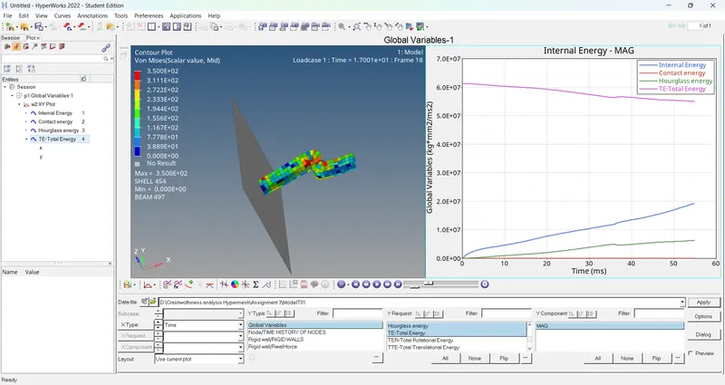
5. Then open 'HyperGraph 2D' in new window. Then browse T01 file as data file. Then select global variables and select energy type as Internal Energy, Contact Energy, Hourglass Energy and Total Energy. Then select magnitude and click on apply. Then select unit profiles as mm, ms and kg and click on ok. The energy graph is plotted.
6. Then for rigid wall forces graph, select rigid wall option and select '4 RIGID WALL1' option. Then select magnitude and normal and tangent forces. Then select unit profiles as mm, ms and kg and click on ok. The graph is plotted.

Case 2: Simulation with improved shell elements properties.

1. Import the solver deck and import the starter(0000.rad) file.
2. Go to 'properties' in browser menu and select the 'component'. Enter the values in entity editor as follows Ishell=24, Ismstr=2, Ish3n=2, N=5, Ithick=1, Iplas=1. And save the model.
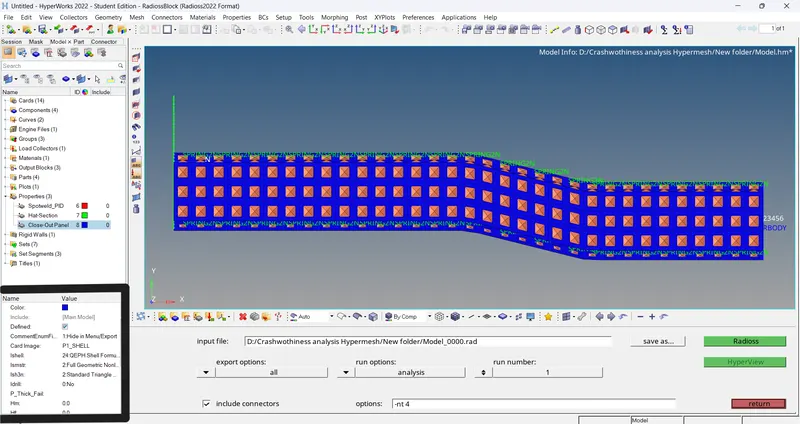
3. To run simulation, Go to 'Analysis' panel and select 'Radioss' option. Ensure the input file and select 'export option' and 'run option' as 'all' and 'analysis' resp. Then enter '-nt 4' in options and click on 'radioss'.
4. After click on radioss, 'compute console solver view' window is open. Then check the energy error and click on 'Results'. And the hyperview window is opened. Select '.h3d' file in 'load model' and 'load result' option and click on apply.
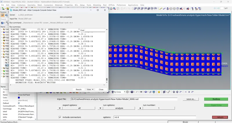
5. Then enable shaded elements and mesh lines. After that click on contour and select result type as 'Von Mises(s)' and hit on apply. Then click on page window layout and select 'split the window in 2 parts'.
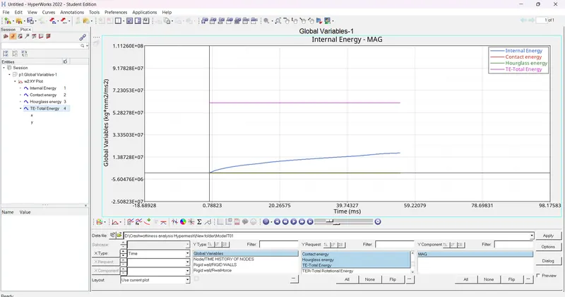
6. Then open 'HyperGraph 2D' in new window. Then browse T01 file as data file. Then select global variables and select energy type as Internal Energy, Contact Energy, Hourglass Energy and Total Energy. Then select magnitude and click on apply. Then select unit profiles as mm, ms and kg and click on ok. The energy graph is plotted.
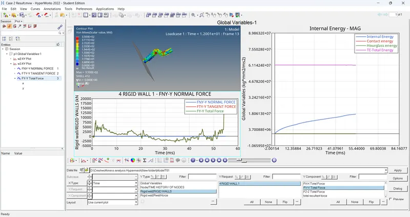
7. Then for rigid wall forces graph, select rigid wall option and select '4 RIGID WALL1' option. Then select magnitude and normal and tangent forces. Then select unit profiles as mm, ms and kg and click on ok. The graph is plotted.

Result:
Case 1:
Error is negative, it means that some energy has been dissipated. The total energy error is decreasing. And Internal energy error and hourglass energy error is increasing. If the error is increases then computation problem is occurs.

Case2:
The total energy error is remains constant so hourglass energy error is constant. It means the computation is much more accurate.

Conclusion: We simulate the model and compare both cases successfully.

Hourglass Energy:
1. Hourglass modes are non-physical modes of deformation that occurs in underintegrated elements and produce no stress.
2. Reduced integration can lerad to non-physical zero energy modes, called hourglass modes.
3. Hourglass modes: A]Kosloff and Frasier Formulation.
B]Flanagan-Belytschko Formulation.
C]Physical Hourglass Formulation.
4. Methods are used to control formation of hourglassing.
A] Perturbation method.
B] Physical stabilization.