Assignment 3-2D Element Formulation Challenge

Crash Beam Simulation and comparison of results with different shell formulations in Radioss.

1. Introduction

Radioss is a widely used explicit solver suitable for highly nonlinear transient simulations. The crash simulation is one such simulation where large deformations take place within 100-300 mili-seconds. In any solver, the input file is a solver deck file from a preprocessing tool like Hypermesh or ANSA. This file contains the mesh and connection data primarily. Further, the material data and properties can be added to the preprocessor as well as the solver. The same is the case with boundary conditions. Various solution controls are applied to the model in the form of different control cards like /Run - which controls the termination time of the simulation.

In Hyperworks the post-processing tasks are mainly performed in the Hyperview and Hypergraph. Hyperview is used for looking at the contours and animation while hypergraph enables the user t plot different results like stress-strain curve, Force-displacement curve etc.

In this exercise, a solver output file for a crash beam and rigid wall was provided. It was asked to run two simulations; one with default shell parameters in the property card and another with all the parameters being set to recommended values. It was expected to draw a comparison of results obtained using the two methods.

2. The model

The geometry consists of a hat section and a close-out section joined together with spot welds. Shell meshing is used for both the members and spring 2N 1D elements are used for modelling the spot weld. Further, a rigid body spider is used at the rear end of the model. A rigid wall is modelled and is positioned in the front of the crash beam as shown in the attached figure.

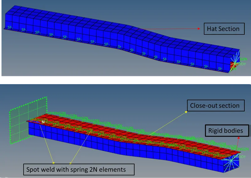
Fig 2.1: The geometry used for the model

An initial velocity of 15.6 mm/ms was applied in the negative X direction so that the beam crashes into the rigid wall. The material used for all the components was steel modelled with a JOHNSON-COOK / ZERILLI-ARMSTRONG ELASTOPLASTIC material card as shown in the below-given image. The unit system followed is [gram-mm-ms].

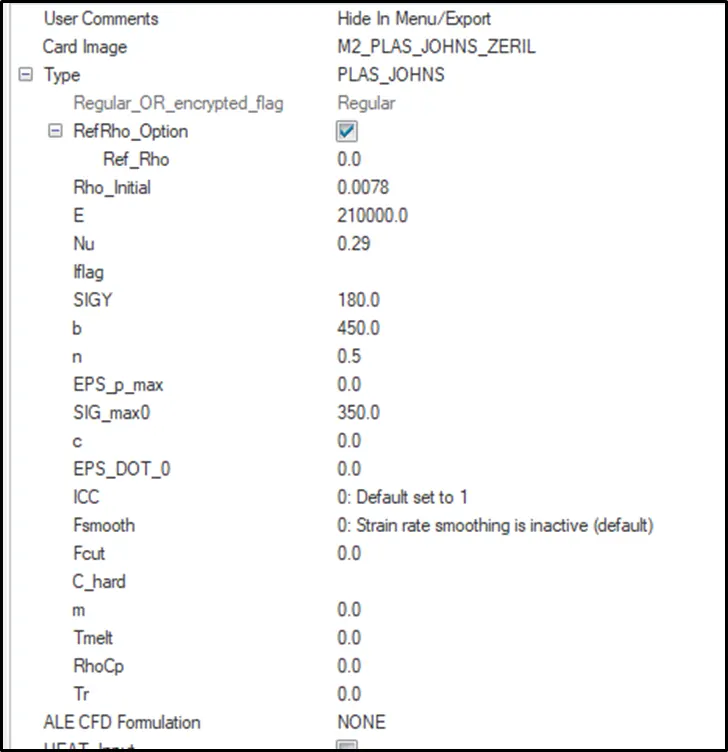
Fig 2.2: The material card used in the model

All other control cards were modelled to control the simulation, a runtime of 55ms was given and total 30 numbers of animation steps were requested by assigning values to the respective cards. proper contact cards were used to avoid elements penetrating into each other during deformation.

2.1 Shell properties

Shell elements need proper property assigned to them in order to get correct results. The calculation of timestep size is dependent on the element size and it can vary with the following :

1. Shell formulation
2. Hourglass control parameters
3. Numerical damping
4. Membrane damping

Radioss provides both reduced and fully integrated 4 noded shell elements and 3 noded tria elements. The selection of different parameters calls for a compromise between cost and speed of simulation. Hourglass refers to the scenario in which a reduced integration element formulation fails to capture the deformation properly. Integration points are the points inside of an element other than nodes that are used for interpolation of the results. In reduced integration elements typically, a single integration point is present at the centre of the element. In the event of bending, this point does not come into the deformation line and the deformation fails to be reported leading to non-physical zero-energy modes also known as hourglass modes.

Similarly, there are other aspects of controlling different parameters for getting an optimised result out of a simulation. Some of them are listed below:

S.N.	Parameter	Comment
1.	Ishell = 24	QEPH 4 noded shells are the best combination of cost and accuracy
2.	Ismstr=2	small strain parameter - Full geometric non-linearity with possible small strain formulation activation
3.	ISH3n=2	(For tria elements)- Standard 3 noded (CO) with modification for large rotations.
4.	N=5	No of integration points set to 5 for accuracy in bending
5.	Ithick =1	Thickness change is taken into account for accuracy.
6.	Iplas =1	Iterative plasticity for better accuracy

In this exercise two simulations were run; one with all of these parameters set to default values and another with all of them changed according to the above table. The results are discussed in the below section. They are named Base run CrashBox and Improved crashbox.

3. Results and discussion

Animation 3.1: the crashing of the crash beam

The beam starts to deform from the sections with geometry change as clear from the animation. Further, energy error and mass added were checked using the .out files written by the solver. Artificial energy addition in the model sometimes leads to a spike in internal energy. This is mainly due to hourglass damping or mass scaling used in the model. A good simulation should keep the % energy error in the range of 0-5% however in some cases it can be allowed up to 10%. Similarly, the mass error should also be checked for any unusual values which are signs of defects in the model.

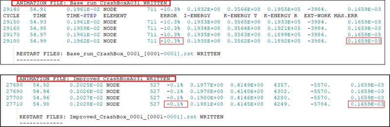
Fig 3.1: the comparison of energy and mass errors

The energy error in the base run was about 10% which indicates a lot of inadequacies in the model. On the other hand, in the improved simulation, it dropped to 0.1% while the simulation time was almost the same for both the runs.

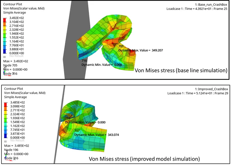
Fig 3.2: the contours of Von Mises stress

A much smoother contour can be observed in the improved run simulation. Gradient formation is easily visible in the baseline simulation result even after using the averaging. The maximum stress values reported are similar in round figures but the big difference is in the smoothness and reporting of the gradient.

Next, Hypergraph was used to plot various parameters for the simulations. They are discussed one by one.

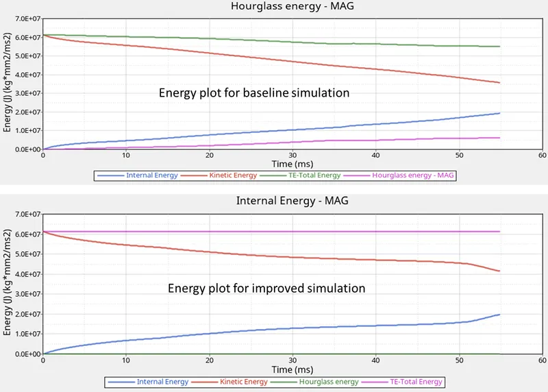
Fig 3.3: Plot of global energies for the simulations

As clear from the above figure, the shape of energy plots confirms the typical crash test plots in which initially high KE due to velocity begins to decrease after contact while the initially low IE begins to rise as the strain energy begins to form as a result of the deformations. The difference, however, can be observed in the sharpness or slopes of curves, they are converging more sharply in the baseline simulation leaving large room for errors during calculations. Also, the hourglass energy can be seen in the baseline simulation which again accounts for the energy error reported in the .out file.

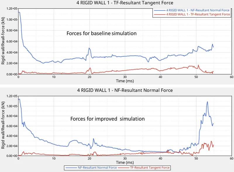
Fig 3.4: the plot of different forces

As apparent from the plots, the normal resultant forces are higher in the baseline simulation, which points out to lesser damping of imbalanced forces and errors in the calculations. The initial high value begins to die down as a result of deformation happening in the beam sections. Also, the friction force is lower in the improved simulation which indicates the proper working of the modelled contacts.

4. Conclusion

• Proper modelling of element formulation is vital for obtaining more accurate simulation results.
• There is a slight increase in the simulation time when all the improvements are made in the shell properties.
• The averaging used in contour gives a more smooth contour which can be used for identifying the high-stress zones in the model.