Assignment 3-2D Element Formulation Challenge

Objective:- The primary objective of this assignment is to compare two simulations with different shell element properties. The comparison would be between the one with default properties and one with the following properties:

Ishell =24		QEPH 4 nodes shells are best combination of cost and accuracy.
Ismstr=2		Full geometric nonlinearities (default)with possible small strain formulation activation in RADIOSS Engine.
Ish3n=2		Standard 3 noded shell (C0)with modification for large rotation(default)
N=5		Number of integration points set to 5 for accuracy bending.
Ithick=1		Thickness change is taken into account for accuracy.
Iplas=1		Iterative plasticity for good accuracy.

Procedure:-

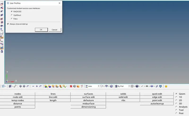
• First step we have to do is to change the user profile to the Raddioss profile, After converting to the Radioss mode we have to import the given starter file (0000.rad) to the hypermesh GUI.

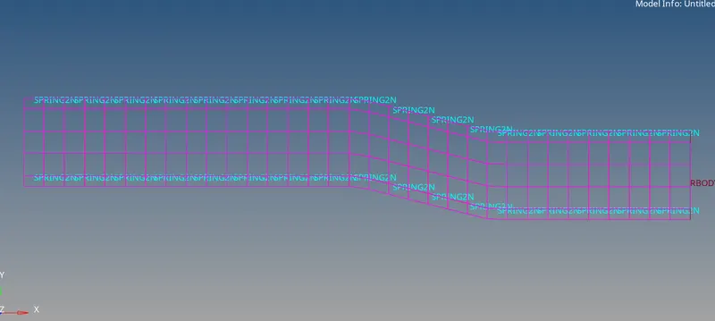
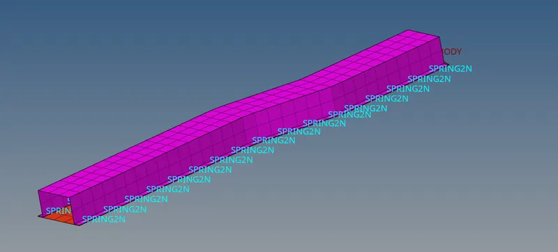
• After importing the file we will see given model in wire frame mode we have to change it to the shaded element and mesh line mode.

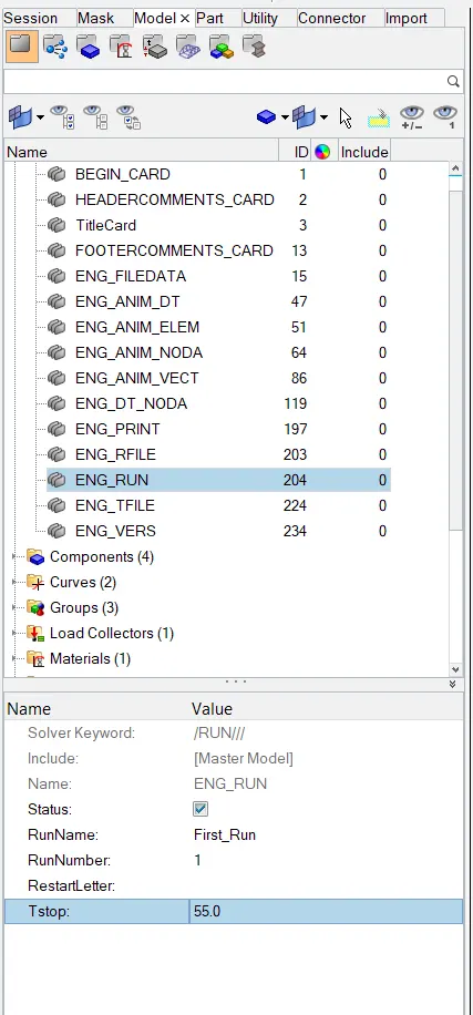
Q.1) change the run time:-

• To change the run time of simulation to 55ms we need to proceed to the solver tab in the side bar by using (Solver deck - Engine keywords - Run - Engine run - Change the Tstop value(55)).

Q.2) Change the number of animation steps during simulation to a minimum of 25 and maximum of 60:-

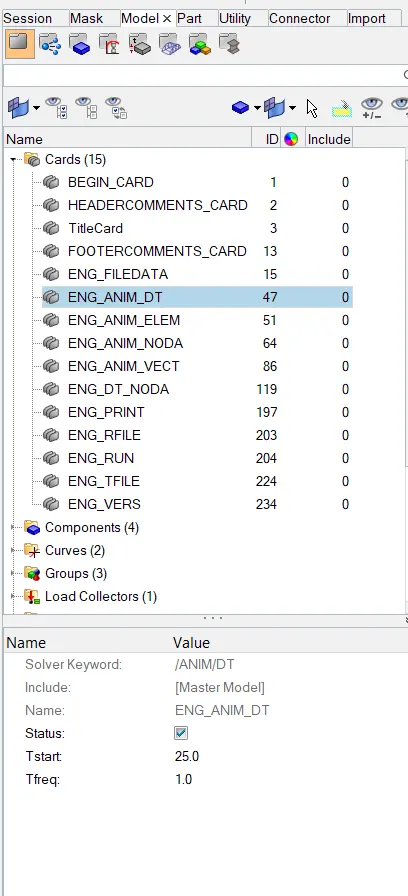
• To change the number of annimation steps during simulation we need to proceed to the solver tab in the side bar by using (Solver deck - Engine keywords - Run - Engine run - ANIM - ANIM\DT - Set the Tstart value and Tfrq value).

Q.3) Run the base simulation:-

• Before run the simulation we have to assign the location to the files which will create after simulation, for this we have to create new folder for that.
• Before going for simulation we have to update some values like we have to tick the inclide connector tab and fill the option space as -nt(space)4. Also select the possition of file in save as option then go for Radioss.

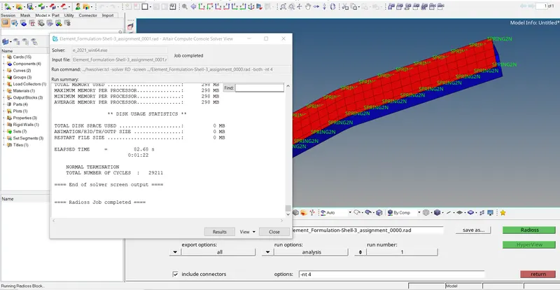
• After completing the simulation it will pop up the chart which shows that our simulation has completed.
• Now by click on result, it will open h3d file which was formed during the simulation which directly take us to hyperview interface then we click on apply.

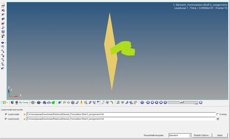
• It will generates the simulation annimation whichever done at the time of simulation, Now we will open it to the contour option in the tool bar.

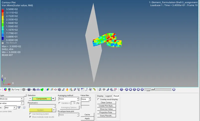
• The given annimation shows von mises

Q.4) To check the energy error and mass error

• To check this we have to open output file (0001.rad) which is created in the folder which we created before simulation.

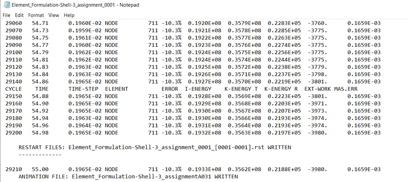
• In that file we will get all the information about enerrgy error and mass error, Also compare it with standard value which is required.

Q.5) Plot the graph of different energies.

• To plot the graph we have to change hypermesh GUI to the Hypergraph 2D GUI. In this we will import the T01 file which is created at the time simulation in the folder which was created before simulation.

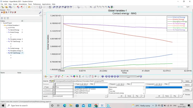
• After adding it, we can select the variables which goes with time.
• First we can go with all the energy graphs.
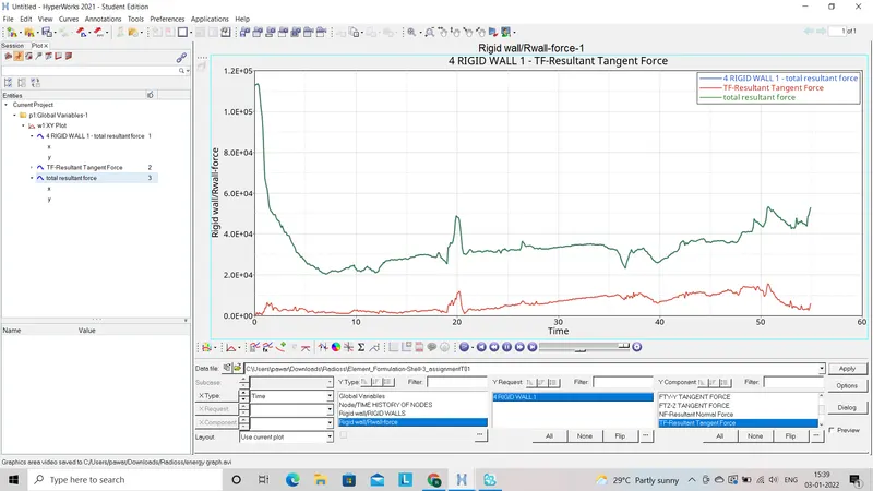
• Now we will generate the graph of rigid wall forces.

Q.6) Change all the shell element properties as per given criteria.

• For this case also we will import the file with same values of Tstop value and annimation step value as same as case 1.
• After that we will go to the model deck to change shell element properties in properties sub menu in that 'Hat section' and 'Close-out panel'.

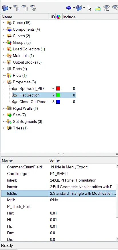
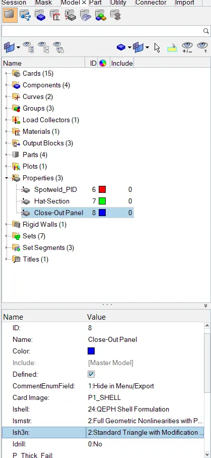
• After changing all the properties of the shell elements we will go to run the simulation.
• Before run the simulation we have to assign the location to the files which will create after simulation, for this we have to create new folder for that.
• Before going for simulation we have to update some values like we have to tick the inclide connector tab and fill the option space as -nt(space)4. Also select the possition of file in save as option then go for Radioss.

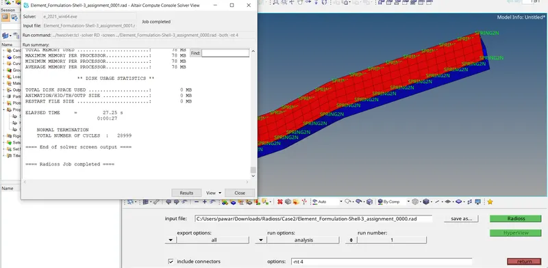
• After completing the simulation it will pop up the chart which shows that our simulation has completed.
• Now by click on result, it will open h3d file which was formed during the simulation which directly take us to hyperview interface then we click on apply.

• It will generates the simulation annimation whichever done at the time of simulation, Now we will open it to the contour option in the tool bar.

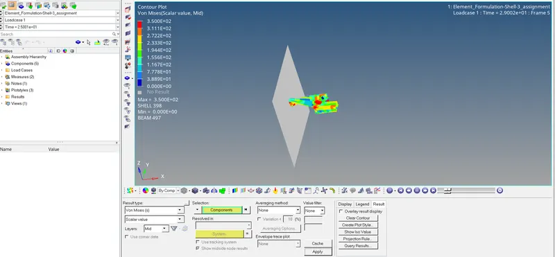
• The following annimation shows von mises
• To check this we have to open output file (0001.rad) which is created in the folder which we created before simulation.

• In that file we will get all the information about enerrgy error and mass error, Also compare it with standard value which is required.

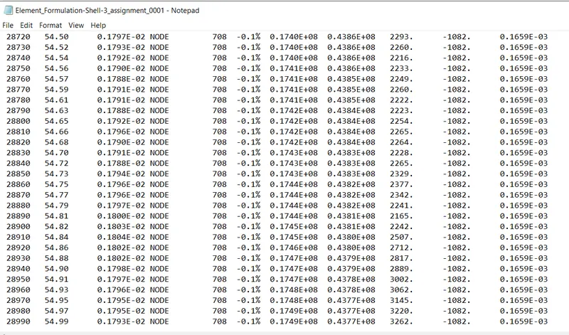
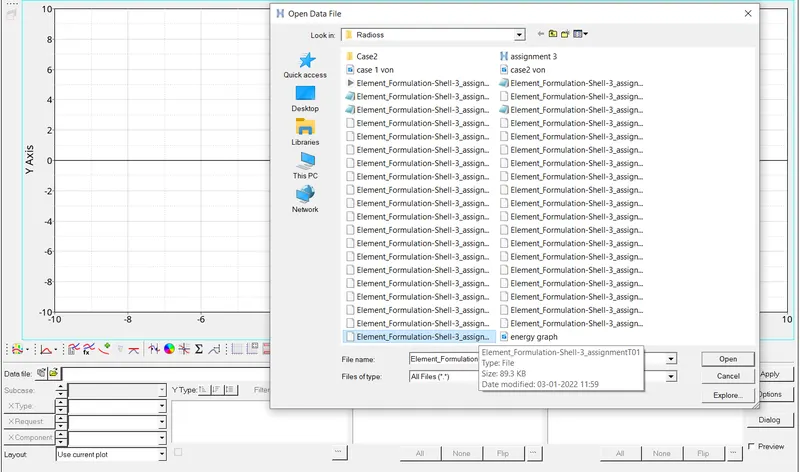
• To plot the graph we have to change hypermesh GUI to the Hypergraph 2D GUI. In this we will import the T01 file which is created at the time simulation in the folder which was created before simulation.
• After adding it, we can select the variables which goes with time.
• First we can go with all the energy graphs.

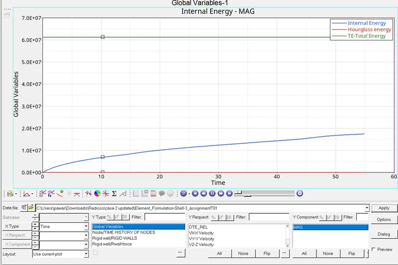
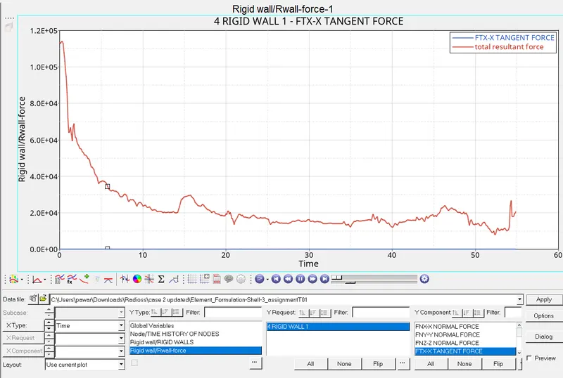
• Now we will generate the graph of rigid wall forces.

Hourglass:-

• Hourglass ia a condition where the elements get deformed but stresses are not get recorded. In short it uncounted energy in the element. as stresses are not produced properly so it reduces the accuracy and behaviour during the simulation.
• To reduce hourglass their are mainly two methods called as

1)Perturbation method

2) Physical stabilization

• In perturbation method forces are applied in opposite direction to stabilize the hourglass. Energy devloped in this process is called hourglass energy.
• In physical stabilization method ues only QEPH elements only. It controls the hourglass from material level.
• Physical stabilization method is better in both the methods as it can use in all kinds of loads.

Results:-

• After comparing both the cases, hourglass energy behaviour is different in both the case.
• Also total energy, rigid wall forces gets different behaviour in both the cases.
• Deformation in beam is more in case 2 compare to case 1.

Conclusion:-

In this challenge I learn about how to run the simulation for given model. Also compare the behaviour of the beam in both the cases.