Comparison of results with base simulation and improved shell element properties for crash analysis in Radioss
Objective:
Compare the results for crash simulation with the default and improved element properties using Radioss solver.
Tasks to be performed:
- Using the given crash beam file, change the run time to 55 ms.
- Change the number of animation steps during simulation to a minimum of 25 and a maximum of 60.
- Run the base simulation without any modification to element properties.
- At the end of the simulation, do the energy error and mass error checks and determine whether the results would be acceptable.
- If acceptable, Plot rigid wall forces, internal energy, hourglass energy, contact energy, the total energy of the simulations.
- Change all the shell elements properties to recommended properties, save this as separate, rad files, and run the simulation.
- Follow steps 5 and 6.
- Compare all the results from steps 5 and 6 for both simulations.
- Comment whether there is any change in the results and why there is any change in the result.
Software used: Hypermesh with Radioss
Introduction:
In finite element methods, calculating the element stiffness is of fundamental importance to computing the deformation of the element, which is done by numerical integration methods. Most of the FEA solvers including Radioss uses the Gaussian quadrature method for finite element calculations. For the function to be integrated, a number of points are considered on the element knows as Gaussian coordinates. For a shell element, in full integration, there are four integration points on the element surface, and in the reduced integration method, there is only one integration point on the element surface. Clearly, the more the number of integration points, the more is the accuracy of the results.
But the fully integrated elements come with a heavy penalty in terms of computation cost. While reduced integrated elements dramatically decrease the computational cost compared to the fully integrated elements. But are less accurate and suffers from hourglassing error.
Hourglass
Hourglass is a weird mode of deformation that occurs in reduced integrated elements and no stresses will be produced. This can affect solution accuracy by varying the structure’s true response. This leads to inaccurate stress, strain, and deflection results. For a reduced integrated element, displacements and forces may exist for each node of the element. If the sum of all these forces and displacements give null strain and stress on the integration point of the element then that element fails to calculate stiffness for certain mode of deformation. At this stage, we say the element has entered into an hourglass mode. Soon after this as the element failed to calculate stiffness the element will behave weirdly.
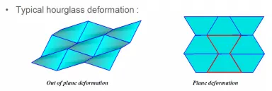
Why does hourglassing happen?
Consider a single reduced-integration element modeling a small piece of material subjected to pure bending (Fig.2)
Neither of the dotted visualization lines has changed in length, and the angle between them is also unchanged, which means that all components of stress at the element's single integration point are zero. This bending mode of deformation is thus a zero-energy mode because no strain energy is generated by this element distortion. The element is unable to resist this type of deformation since it has no stiffness in this mode. In coarse meshes this zero-energy mode can propagate through the mesh, producing meaningless results.
How is hourglassing controlled?
- By inserting an artificial stiffness to the hourglass deformation modes (the default way utilized in static/quasi-static problems).
- By inserting an artificial viscosity (preferred for dynamic and high-velocity impact problems).
- By using fully integrated elements.
Element formulation in Radioss
Radioss provides both reduced and fully integrated 4-noded shell elements.
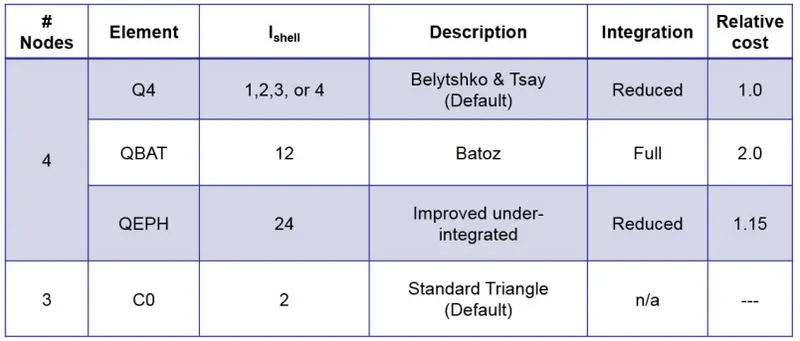
Two methods used to control the formation of hourglassing:
- Perturbation (Q4 Elements)
- Physical Stabilization (QEPH Elements)
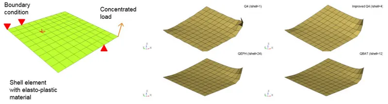
Hourglass Perturbation Control Method
- Perturbation method Ishell=1,2,3 or 4 (Q4)
- The hourglass deformation is detected with the relative motion (velocity) of the nodes.
- When hourglassing is detected, a force is applied to the node to stabilize the deformation.
- This force is defined according to the element stiffness (Young modulus, yield stress, plastic tangent, ..)
- This force introduces an artificial energy (named hourglass energy)
- Perturbation method Ishell= 24 (QEPH)
- Hourglass yield depends on the natural yield
- Hourglass loading stiffness depends on the natural tangent modulus
- The hourglass treatment is done at the material level
Procedure:
First, the solver deck file is imported into the Hypermesh-Radioss workspace. The image below shows the model setup for simulation,
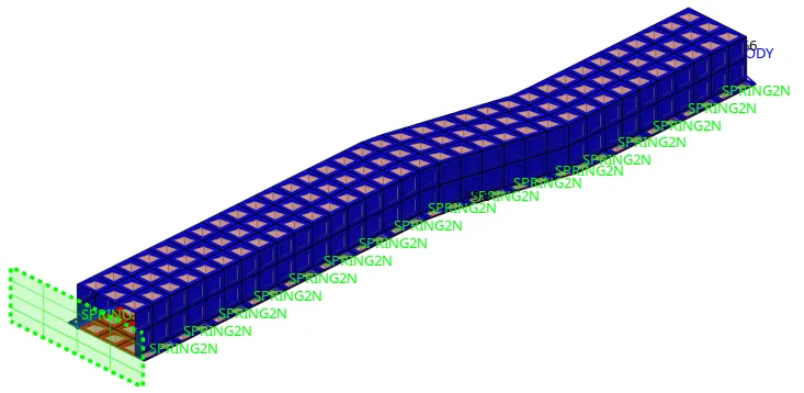
For this simulation, a crash tube is used made up of two parts, spot welded together. At the end of the tube, a cluster of rigid body elements is deployed and mass is applied to the master node. An initial velocity is given at the master node to crash the tube with the rigid wall.
After importing the model, the run time is changed from 60ms to 55ms by going to Model tree>Cards>ENG_RUN. The same can be done by directly editing the engine file (_0001.rad ).
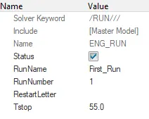
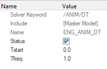
The next task is to change the number of animation steps during simulation to a minimum of 25 and a maximum of 60. The number of animation steps can be changed by going to Model tree>Cards>ENG_ANIM_DT. There, the parameter 'Tfreq' is equal to the termination time divided by the number of animation steps. Therefore, the value of Tfre is kept at 1, which corresponds to 55 animation steps.
Case 1:
Next, base simulation is run by going to Analysis>Radioss.
Time to solve: 31.68s
After running the simulation, energy error and mass error is checked in the 'xxxx_0001.out' file, as shown in the image below.
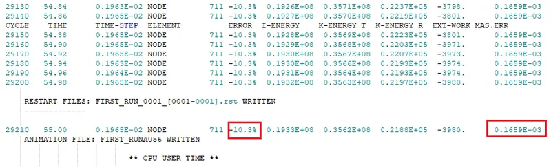
The energy error is -10.3% and the mass error is 0.1659E-03.
Radioss computes the energy error as a percentage. A negative error means that some energy has been dissipated. And, for reduced integrated elements, this is because of Hourglass energy. An energy error of less than -15% is considered acceptable for simulation results.
The simulation results are acceptable as the energy error is increasing gradually and is less than -15% and, the mass error is also very less.
Next, switch to the Hyperview workspace and open the .h3d file. The animation below shows the displacement.
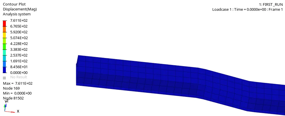
We can see that most of the element deformations are not natural. This is because of the reduced integrated elements used. The solver fails to properly calculate the deformation and stress for the elements.
Next, to plot the results switch to HyperGraph 2D workspace and open the data file 'xxxxT01'. First, the contact forces are plotted as shown in the image below.
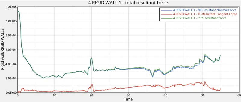
As expected, the normal force is very high during the start of impact and then decreases and then again increases during the end when rear-end crashes with the wall. Also, the friction force is increasing as the contact surface area of the crash tube with the rigid wall is increasing during the simulation.
Next, internal energy, hourglass energy, contact energy, the total energy of the simulations are plotted as shown in the image below,
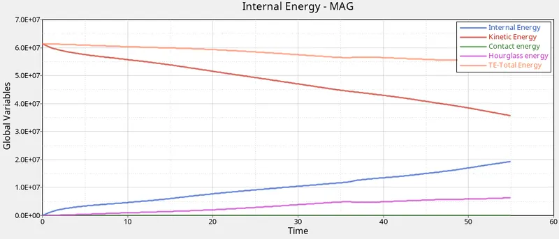
From the plot, we can see, at the start of the simulation, kinetic energy was maximum and internal energy was zero. And, with time, kinetic energy is decreasing and the internal energy is increasing due to strain, as expected.
Total energy should have been constant and stable but it is also decreasing and the hourglass energy is increasing which is not ideal.
Case 2:
For the second simulation, the following recommended element properties were used,
| Parameters | Comment |
|
Ishell =24 |
QEPH 4 nodes shells are best combination of cost and accuracy. |
|
Ismstr=2 |
Full geometric nonlinearities (default)with possible small strain formulation activation in RADIOSS Engine. |
|
Ish3n=2 |
Standard 3 noded shell (C0)with modification for large rotation(default) |
| N=5 | Number of integration points set to 5 for accuracy bending. |
|
Ithick=1 |
Thickness change is taken into account for accuracy. |
|
Iplas=1 |
Iterative plasticity for good accuracy. |
The above properties were configured for both 'Hat_section' and 'close_out_panel' by going to Model tree>Properties.
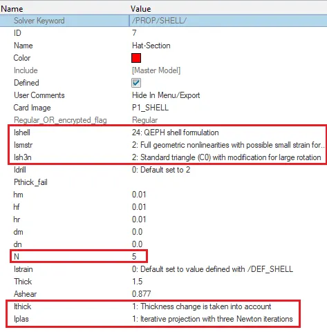
Next, the simulation is run by going to Analysis>Radioss.
Time to solve: 37.71s
After running the simulation, energy error and mass error is checked, as shown in the image below.
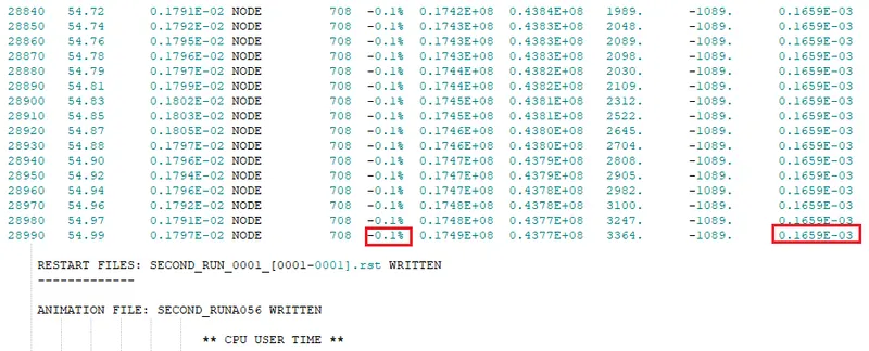
The energy error is -0.1% and the mass error is 0.1659E-03.
In the case of using QEPH shell formulation (Ishell=24) or fully integrated elements, the Energy Error can be slightly positive since there is no Hourglass energy and the computation is much more accurate. An error of +1% or +2% is acceptable. If the error is positive, there is an energy creation.
The simulation results are acceptable as the energy error is less than -15% and, the mass error is also very less.
Next, switch to the Hyperview workspace and open the .h3d file. The animation below shows the displacement.
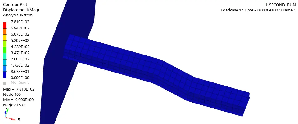
We can observe that the element deformations are much more realistic than in case 1.
Next, to plot the results switch to HyperGraph 2D workspace and open the data file 'xxxxT01'. First, the contact forces are plotted as shown in the image below.
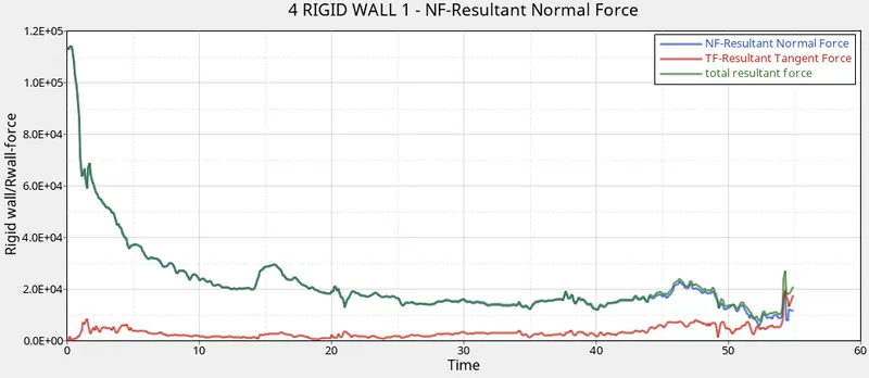
As expected, the normal force is very high during the start of impact and then decreases and then again increases during the end when rear-end crashes with the wall. Also, the friction force is increasing as the contact surface area of the crash tube with the rigid wall is increasing during the simulation.
Next, internal energy, hourglass energy, contact energy, the total energy of the simulations are plotted as shown in the image below,
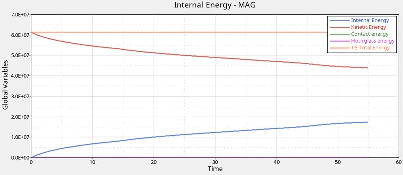
As expected, we can observe that at the start of the simulation, kinetic energy was maximum and internal energy was zero. And, with time, kinetic energy is decreasing and the internal energy is increasing due to strain.
The total energy is also stable during the simulation and hourglass energy is zero. Therefore, the results obtained are much more accurate.
Conclusion:
The simulations with the default and improved element properties were successfully done.
The simulation with improved element properties took more time to solve than in case 1, considering it was a fairly simple simulation setup.
The energy error was also less and much more ideal in case 2 than in case 1. Total energy remained constant in case 2 and hourglass energy was also zero. Therefore, the results in case 2 are much more accurate than in case 1.
Therefore, we can conclude that the improved element properties with QEPH element formulation are a better choice for crash simulations giving a good compromise between computational cost and accuracy.