Analyse the Pipe Flow Simulation with an Inlet velocities of the water with different inlet Reynolds number.

AIM :- To Analyse the Pipe Flow Simulation with an Inlet velocities of the water with different inlet Reynolds number.

COMPUTATIONAL FLUID DYNAMICS (CFD) :-

Computational fluid dynamics (CFD) is a branch of fluid mechanics that uses numerical analysis and data structures to analyze and solve problems that involve fluid flows. Computers are used to perform the calculations required to simulate the free-stream flow of the fluid, and the interaction of the fluid (liquids and gases) with surfaces defined by boundary conditions. With high-speed supercomputers, better solutions can be achieved, and are often required to solve the largest and most complex problems. Ongoing research yields software that improves the accuracy and speed of complex simulation scenarios such as transonic or turbulent flows. Initial validation of such software is typically performed using experimental apparatus such as wind tunnels. In addition, previously performed analytical or empirical analysis of a particular problem can be used for comparison. A final validation is often performed using full-scale testing, such as flight tests.

CFD is applied to a wide range of research and engineering problems in many fields of study and industries, including aerodynamics and aerospace analysis, weather simulation, natural science and environmental engineering, industrial system design and analysis, biological engineering, fluid flows and heat transfer, and engine and combustion analysis.

Methodology:-

In all of these approaches the same basic procedure is followed.

During preprocessing

• The geometry and physical bounds of the problem can be defined using computer aided design (CAD). From there, data can be suitably processed (cleaned-up) and the fluid volume (or fluid domain) is extracted.
• The volume occupied by the fluid is divided into discrete cells (the mesh). The mesh may be uniform or non-uniform, structured or unstructured, consisting of a combination of hexahedral, tetrahedral, prismatic, pyramidal or polyhedral elements.
• The physical modeling is defined – for example, the equations of fluid motion + enthalpy + radiation + species conservation
• Boundary conditions are defined. This involves specifying the fluid behaviour and properties at all bounding surfaces of the fluid domain. For transient problems, the initial conditions are also defined.

• The simulation is started and the equations are solved iteratively as a steady-state or transient.
• Finally a postprocessor is used for the analysis and visualization of the resulting solution.

Pipe Flow

Flows completely bounded by solid surfaces are called INTERNAL FLOWS which include flows through pipes, ducts, nozzles, diffusers, sudden contractions and expansions, valves, and fittings. Based on the values of a non-dimensional number known as Reynold’s number (Re), the flow in the pipe can classified.

The Reynold’s Number (Re) is defined as the ratio of Inertia force of a flowing fluid and the
Viscous force. It is mathematically expressed as,
Re=(Inertia force/Viscous force) =( ρ V D/µ )
Where, ρ is mass density
V is average velocity of flow
D is diameter of pipe
µ is dynamic viscosity of flowing fluid
Based on the values of Reynold’s number (Re), flow is classified as Follows:

Laminar flow Occurs when Reynold’s number Re< 2000.

In laminar flow velocity increases gradually from zero at the boundary to Maximum at the center. Laminar flow is regular and smooth and velocity at any point practically remains constant in magnitude & direction. Therefore, the flow is also known as stream Line flow.

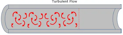
Turbulent flow occurs when Reynolds number above 4000.

In the turbulent flow the fluid flow at higher flow rates, the streamlines are not steady and straight and the flow is not laminar. Flow is very much disorder and there will be violent mixing.

Transitional Flow

In this, the condition is neither the laminar nor turbulent. It is intermittently turbulent flow. The stream lines get disturbed a little.
This type of flow occurs when 2000< Re < 4000.

INPUT DATA AND GOVERNING EQUATIONS :-

• Diameter of Pipe = 0.02m (ID)
• Thickness of Pipe = 0.002m
• Length of Pipe = 1m
• Fluid :- Water @ Re = 100, 1000, 10000
• Density of Water = 1000Kg/m^3
• Consider Outlet Pressure & Temperature :- 101325 Pa, 293K

Dynamic viscosity Ns/m^2 (also known as absolute viscosity) is the measurement of the fluid’s internal resistance to flow while kinematic viscosity...m^2/s refers to the ratio of dynamic viscosity to density.

Kinematic Viscosity of Water at 293K = 1.004*10^-6 m^2/s

% CALCULATIONS

Re = [V.D]/v
V = [Re.v]/D
V = [100*1.004*10^-6]/0.02
V=‭0.005020

So, The 3 different Velocities at 3 different Reynolds Numbers are given as follows,

%Re       %V(m/s)

100      0.005020
1000     0.05020
10000    0.5020

PROCEDURE OF SIMULATION :-

Create the Pipe Model as per the data given below.

• Diameter of Pipe = 0.02m (ID)
• Thickness of Pipe = 0.002m
• Length of Pipe = 1m

Then we will Form Lids on the both sides of the walls of the Pipe from the Flow Simulation>create Lids

Now, Place line probes at 95%, 90% and 85% of the pipe length by inlet by drawing Sketches.

Now, Create the new Project in Flow Simulation.

And Click on the wizard panel to create General Settings in our flow Simulation.

In General settings, in the initial conditions select the water as a Fluid of Laminar and Turbulent type.

Now, Insert the Boundary Conditions

1. @ the Outlet of the Pipe, Static Pressure of 101325 Pa & 293.2k Temp
2. @ the Inlet of the Pipe, any Velocity obtained from above all 3 cases.
3. @ the Inner Wall of the Pipe, Real Wall.

Now, Create the Basic Mesh and then edit the definitions of the Global Mesh by selecting Manual type and set 10 @ X-direction, 10 @ Y-direction, 50 @ Z-direction (since flow is in Z-direction. Also enable the Advance Refinement.

And Insert XY Plots at the 3 different Line Probes drawn earlier.

Then Create Cut Plots to check the Inner flow clearly of all three line probe which are made earlier using Front plane.

And Also Create Another Cut plot in Right plane to see whole inner Flow of the Pipe.

Create a New Parametric Study, Add Simulation Parameters in Input Variables. Then select the Boundary Conditions :- Inlet Velocity and add Normal to Face Parameter.

Select the Output Parameters and select all XY Plots & Cut Plots.

Create 2 new design points and change the Inlet Velocities which we had earlier.

RUN the Simulation and Evaluate the Results.

RESULTS :-

Case 1 : When R = 100 :-

Cut plot & Velocity profile at 95% :-

Cut plot Velocity profile at 90% :-

Cut plot & Velocity profile at 85% :-

Cut plot of Whole pipe :-

Case 2 : When R = 1000 :-

Cut plot & Velocity profile at 95% :-

Cut plot Velocity profile at 90% :-

Cut plot & Velocity profile at 85% :-

Cut plot of Whole pipe :-

Case 3 : When R = 10000 :-

Cut plot & Velocity profile at 95% :-

Cut plot Velocity profile at 90% :-

Cut plot Velocity profile at 85% :-

Cut plot of Whole pipe :-

Case 4 : Velocity Profile Comparison:-

At R = 100 :-

At R = 1000 :-

At R = 10000 :-

Velocity Comparison of all Cases :-

CONCLUSION:

It can be concluded that as we increase the Reynold's Number (from 100 - 1000 - 10000), the velocity increases and has a visible defined red center in the cut plots indicating the gain in velocity.