Air Standard Cycle

Creating a Matlab program for analysing an air standard cycle through P-V diagram.

Report

1. Aim:

• Analysing an Air Standard Cycle through P-V diagram by writing Matlab program for an engine’s power stroke.

2. Theory and Equations & Calculations:

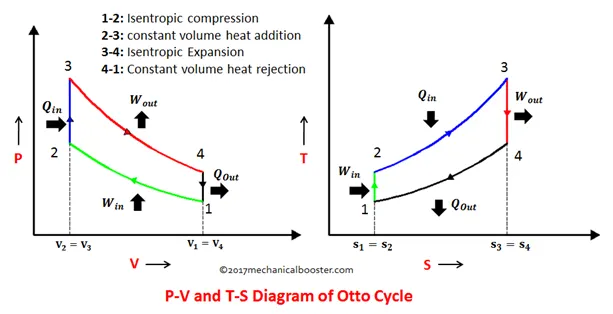
• There are four processes that take place in otto cycle and this cycle is a power stroke. These processes happens in this chronology, first one the isentropic compression then constant volume heat addition then isentropic (reversible adiabatic) compression then constant volume heat rejection.
• Isentropic Processes follows:

`PV^gamma`= constant, which implies that `(p1)/(p2)=((v2)/(v1))^gamma`

Ideal Gas Law/ Boyle’s Law:

PV/T = constant, which implies that `p1*(v1)/(t1)=p2*(v2)/(t2)`

For ideal gas C_p and C_v are constant then `gamma=(Cp)/(Cv)` is taken as input 1.4 for air.

Volume trace:

`V/(Vc)=1+0.5(Cr-1)[R+1-costheta-(R^2-sintheta^2)^(1/2)]`

Where V_c is clearance volume, C_r is compression ratio, `theta` is crank angle

Units used for different parameters:

Length in meters

Temperature in Kelvin

Pressure in kPascal

• Assumption taken while analysing the otto cycle, these assumption are taken to reduce the complexity as a cycle is very much complex.

1. The gas in the cylinder is ideal gas and it is a closed system.
2. The compression and expansion are adiabatic reversible means no heat interaction and no friction.
3. In place of combustion, heat is provided by bringing hot material in contact.

• Cycle Explanation:

1. So the process begins with the piston is at Bottom Dead Centre (BDC) and starting to compress, this compression is isentropic compression so there will be no heat ejection. The pressure and temperature will increase according to the relations from isentropic and Boyle’s law
2. Now there will be constant volume heat addition not by any chemical reaction but it done by bringing hot material basically in real world the combustion happens so fast that to make it simple we take constant volume and instead of combustion we take heat is supplied to the system. So the pressure will increase rapidly keeping the volume constant, with given temperature after combustion we use the Boyle’s law to get the pressure after combustion.
3. After this heat addition there will be isentropic expansion, similarly there will be no heat interaction, the piston will be at BDC again making the volume to be same as of the starting, pressure will also be decreased and can be estimated by the isentropic relation.
4. At last there will be constant volume heat rejection means heat will be come out with the exhaust gases, considered to make the process simpler.

3. Objective:

To create a reference cycle for estimating an engine power, creating a standard for an engine to get rough idea about its performance. We idealise some complex processes to create some standards so to estimate engine performance like for this geometry, compression ratio, combustion temperatures this will be the engine performance, so we can get some estimation for another engine.

Workflow:

• Firstly the cylinder geometry and temperature, pressure parameters at first state are taken as input.
• The parameters at the second state (Isentropic compression) is calculated with above defined relations.
• Similarly the parameters at the state third and fourth are calculated after the cycle reaches its initial state.
• To show the isentropic compression and expansion we find the volume trace, creating a matrix of volume from state 1 to 2 and 2 to 3. According to these volume we calculate the pressure matrix.
• At last plot all these parameters to get the P-V diagram of the otto cycle and then we calculate the thermal efficiency of the engine.

4. Matlab Program:

The programming language used is MATLAB.

%Plotting P-V for an Air Standard Cycle of Hyundai 1 litre T-GDI engine
close all;
clc;

%Cylinder Geomtry
bore=0.071;    %meter
stroke=0.084;  %meter
conn_rod=0.09; %meter
comp_ratio=10;

%Inputsparamters for the cycle
gamma=1.4;  %gamma=Cp/Cv for air taking mass=28;
p1=101.325; %kilo pascal
t1=300;     %kelvin
t3=1500;
%p1,v1,t1 are the parametes at state 1, similarly p1,v2,t2 are the
%paramters at state 2 and so on for state 3 and 4

%Parameters before compression state 1

swept_v=(pi/4)*bore^2*stroke;
clear_v=swept_v/(comp_ratio-1);
v1=swept_v+clear_v;
v2=clear_v;


%Parameter after Isentropic copression state 2

%As in insentropic process
%p1v1^gamma=p2v2^gamma, p2=p1(v1/v2)^gamma
p2=p1*(v1/v2)^gamma;

%Calculating discrete values of P-V from state 1 to 2 from relatioin
%of volume derived from cylinder geometry
constant=p1*(v1^gamma);
compressing_vol=volume_trace(bore,stroke,conn_rod,comp_ratio,180,0);
compressing_pres=constant./compressing_vol.^gamma;

%Gas is assumed to be ideal so boyle's law
%p1v1/t1=p2v2/t2
t2=p2*v2*t1/(p1*v1);

%Parameters after constant volume heat addition state 3
%for that we take input parameter t3 after heat addition or combustion

v3=v2;          %constant volume
%ideal gas obey boyle's law
%p2v2/t2=p3v3/t3, p3=p2v2t3/t2v3
p3=p2*t3/(t2);

%Calculating discrete values of P-V from state 3 to 4 from relatioin
%of volume derived from cylinder geometry

constant1=p3*(v3^gamma);
expanding_vol=volume_trace(bore,stroke,conn_rod,comp_ratio,0,180);
expanding_pres=constant1./expanding_vol.^gamma;

%Parameters after isentropic expansion state 4
%for isentropic pv^gamma=constant
v4=v1;    %as after it, constant volume heat rejection
p4=p3*(v3/v4)^gamma;

%plotting the parameters

hold on;
plot([v1 v2 v3 v4],[p1 p2 p3 p4],'*','color','r');
plot([compressing_vol expanding_vol],[compressing_pres expanding_pres],'color','b','linewidth',1);
plot([v4 v1],[p4 p1],'linewidth',1,'color','b');
xlabel('volume');
ylabel('pressure');

efficiency=1-(1/comp_ratio^(gamma-1));

Code Explanation:

• We take a Hyundai 1.0-litre T-GDI engine, the cylinder geometry (bore, stroke, connecting rod, compression ratio) are taken whereas the parameters for state 1 are taken as input. The pressure and temperature are taken for moderate conditions and the volume is equal to the sum of swept and clearance volume as the piston is at BDC.
• The swept and clearance volume are calculated using the cylinder geometry, as swept volume is the volume which the piston covered from BDC to TDC. The clearance volume is the volume where the combustion will occur and it is one less than compression ratio part of the swept volume.
• So the volume for state 1 and 2 are calculated as volume after isentropic compression will be equal to clearance volume. Then using the relation `(p1)/(p2)=((v1)/(v2))^gamma` we calculate the pressure at state 2, where gamma is taken as input for ideal gas. The temperature is calculated using the relation from Boyle’s law.
• In between we call the function volume trace from which we get matrix of volume as it goes from state 1 to state 2 corresponding to each volume we calculate the pressure accordingly using the relation `PV^gamma`= constant.
• For the state 3 we take temperature as input after the heat addition at constant volume. The heat is added at constant volume means the volume remains the same as of state 2, which takes us to calculate the pressure at state 3 using the relation of Boyle’s law.
• The expansion takes place from state 3 to 4 for which we call the function volume trace again to get the volume matrix of expansion corresponding to which we calculate the pressure matrix.
• At state 4, from where there will be constant volume heat rejection and the goes to initial conditions, we conclude that volume at state 4 and 1 is equal. The process from state 3 to 4 is isentropic expansion which helps us to use the relation to calculate the pressure at state 4.
• At last we start plotting the parameters, to keep all the plots from each command we use the hold on command to show all the plots in one figure.
• The first plot command marked the each state P-V in red colour. The second plot command is used to plot compression and expansion process. The last one is to plot the relation between state 3 and 4.
• Furthermore we calculate the thermal efficiency of the engine using the relation `eta=1-1/((Cr)^(gamma-1` where C_r is the compression ratio.

Function volume_trace code:

function [vol]= volume_trace(bore,stroke,conn_rod,comp_ratio,BDC,TDC)

swept_vol=(pi/4)*bore^2*stroke;
clear_vol=swept_vol/(comp_ratio-1);

crank_pin_radius=stroke/2;
R=conn_rod/crank_pin_radius;

theta=linspace(BDC,TDC,180);

eq1=0.5*(comp_ratio-1);
eq2=R+1-cosd(theta);
eq3=(R^2-sind(theta).^2).^0.5;

vol=(1+eq1*(eq2-eq3))*clear_vol;

end

Explanation:

• In this function we create the volume matrix for the isentropic compression and expansion using the relation stated above for volume trace. In this relation we need different variables to be calculated first as clearance volume and R which remains constant through the process.
• As we go from the BDC to TDC the `theta` is going to vary accordingly which we create a matrix using the linspace command.
• Then we distribute the relation into smaller equations and at last put them together easily.

5. Output:

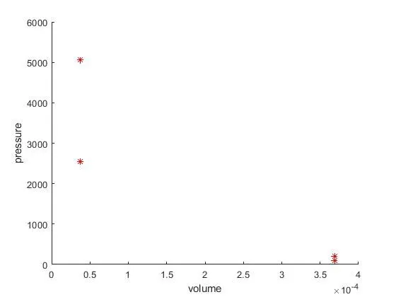
These are the four states of an otto cycle for the different processes.

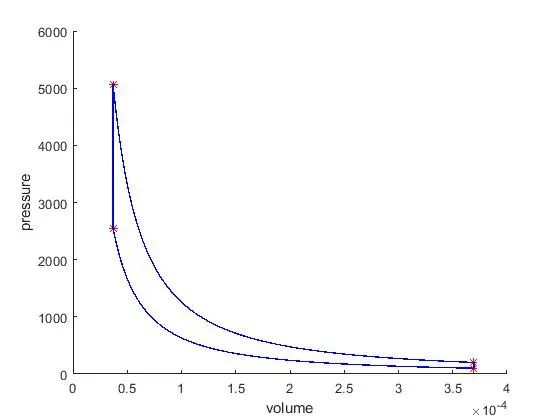
This is the plot for the otto cycle going through the different processes.

6. Conclusion:

• The thermal efficiency of the engine is 60.19% and as we increase the compression ratio the thermal efficiency of the engine will increase.
• We can analyse the pressure and volume at any point of the cycle to get the estimation on how much pressure and volume will change after or before combustion.

7. References:

https://www.youtube.com/watch?v=Da24ckBPK0w

https://web.mit.edu/16.unified/www/FALL/thermodynamics/notes/node26.html