Ahmed Body Challenge
Title: Ahmed Body Challenge
Theoretical Concept:
- Ahmed Body:
The Ahmed body is a benchmark model widely used in the automotive industry for validating simulation tools.
The Ahmed body shape is simple enough to model, while maintaining car-like geometry features.As the burning of fossil
fuels becomes a more pressing issue, manufacturers are introducing more fuel efficient cars to the market. One main
contributor to fuel burn is the car’s aerodynamic drag. Complexly shaped, cars are very challenging to model and it’s difficult
to quantify the aerodynamic drag computationally.
The drag coefficient quantifies the resistance of an object in a fluid environment. It is not an absolute constant for a
body’s shape because it varies with the speed and direction of flow, object shape and size, and the density and viscosity of the
fluid. The lower the drag coefficient of an object, the less aerodynamic or hydrodynamic drag occurs. In terms of a car, the
lower the drag coefficient, the more efficient the car is. As well as affecting the top speed of a vehicle, the drag coefficient also
affects the handling. Cars with a low drag coefficient are sought after, but decreasing the drag drastically can reduce the downforce
and lead to loss in road traction and a higher chance of car accidents.
The Ahmed Body was first created by S.R. Ahmed in his research “Some Salient Features of the Time-Averaged Ground
Vehicle Wake” in 1984. Since then, it has become a benchmark for aerodynamic simulation tools. The simple geometrical shape has
a length of 1.044 meters, height of 0.288 meters, and a width of 0.389 meters. It also has 0.5-meter cylindrical legs attached to the
bottom of the body and the rear surface has a slant that falls off at 40 degrees.
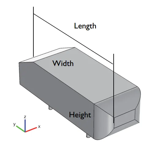
Fig: Simple Geometry of Ahmed Body
The flow for this model is turbulent, which is based on the Reynolds number determined by the body length and inlet velocity. The
simulation solves for the turbulent kinetic energy in addition to the velocity field. For this simulation, we need a larger mesh size than
what is usually common to resolve the turbulent flow. More specifically, we use a finer mesh downstream of the model to capture the
wake zone.The flow for this model is turbulent, which is based on the Reynolds number determined by the body length and inlet velocity.
The simulation solves for the turbulent kinetic energy and dissipation in addition to the velocity and pressure fields.
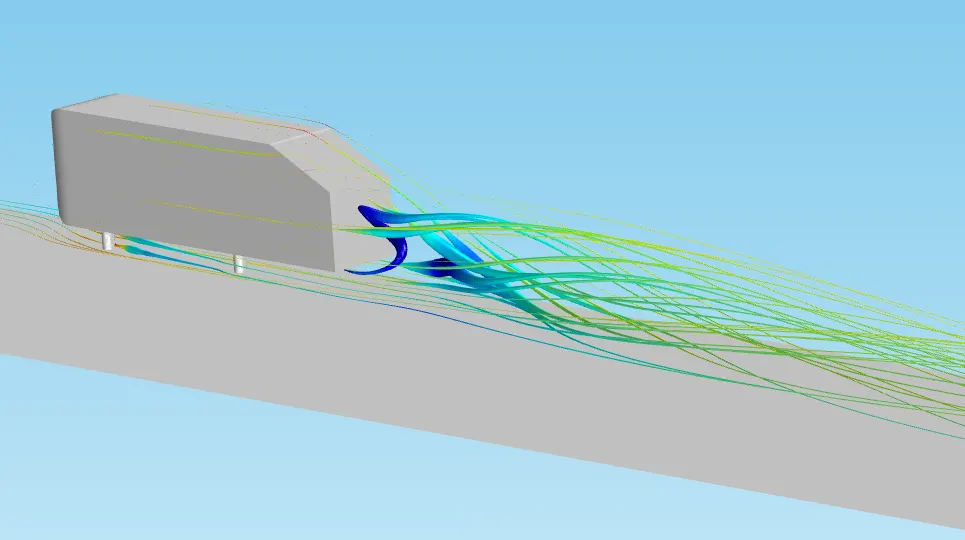
Fig: Streamlines Behind the Ahmed Body
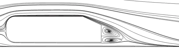
Fig: Recirculation zones past the Ahmed Body
- Importance of Ahmed Body:
* Ahmed body is a benchmark model used in automotie industry for validating simulation tools.
* The Ahmed body shape is simple enough to model, while maintaining car-like geometry features.
* This simulation of Ahmed body is more than adequate for calculating the overall drag coefficient.
* It helps to analyse complex car geometry.
- Negative Pressure in Wake Region:
When the air moving over the vehicle is separated at the rear end, it leaves a large low pressure turbulent region behind the vehicle
known as the wake. This wake contributes to the formation of pressure drag, which is eventually reduces the vehicle performance.
The region of recirculating flow immediately behind a moving or stationary blunt body, caused by viscosity, which may be accompanied
by flow sepration and turbulence flow, or the wave pattern on the water surface downstream of an object in a flow, or produced by a moving
object (e.g. a ship), caused by density differences of the fluids above and below the free surface and gravity.
When the vehicle is moving at a certain velocity, the viscous effects in the fluid arerestricted to a thin layer called boundary layer.
Outside the boundary layer is the inviscid flow. This fluid flow imposes pressure force on the boundary layer. When the air reachesthe rear part
of the vehicle, the fluid gets detached. Within the boundary layer, the movement of the fluid is totally governed by the viscous effects of the fluid.
The Reynolds number is dependent on the characteristic length of the vehicle, the kinematic viscosity and the speed of the vehicle. The fluid moving
around the vehicle is dependent on the shape of the vehicle and the Reynolds number. There is another important phenomenon, which affects the
flow of the car and the performance of the vehicle. This phenomenon is commonly known as ‘Wake’ of the vehicle. When the air moving over the
vehicle is separated at the rear end, it leaves a large low-pressure turbulent region behind the vehicle known as the wake. This wake contributes to
the formation of pressure drag, which is eventually reduces the vehicle performance.
Fig: Flow separation and wake region
- Significance of Point of Separation:
Separation of flow is said to occur when the direction of the flow velocity near the surface is opposed to the direction of the free stream velocity
, which means (du/dy) ≤ 0. Such a situation arises when there is a negative pressure gradient near the wall (Refer Fig.). An example is subsonic
diffuser or rear portion of the car.
In the direction of flow the pressure increases which causes decreases in velocity and creates condition for separation to occur. It is important to
note that, the skin-friction coefficient reaches the value zero. At this point the wall shear stress vanishes is called the separation point. Reverse flow
takes place beyond point of separation. Due to reverse flow, irregular eddies are formed and lot of energy is dissipated. This region is called „Wake‟.
The pressure distribution in the wake is quite different from that on the remaining boundary and this gives rise to an additional drag force on the body.
Wake also leads to lateral vibration to the object which may be harmful. Also large amount of K.E. is lost.
In the turbulent boundary layer, some of the energy is dissipated in friction, slowing airflow velocity, resulting in a pressure increase. If the
increase in pressure is gradual, the process of turbulent mixing will cause a transfer of energy from the fast moving eddies to slower ones in the
turbulent boundary layer. If the rate of change in pressure is too great, for example in sharp corners, the mixing process will be too slow to push the
slower air molecules moving. When this happens, the boundary layer flow stops following the contours of the surface, resulting in separation. Air particles
downstream of the separation region will then move towards the lower pressure region in the reverse direction to the mainflow, the separation region will
reattach. In the region between separation and reattachment points, air flow is circulating and this is called the „separation bubble Separation will normally
occur if the resultant flow encounters a sharp edge and that is why it is always importantfor ground vehicles to have smoothly rounded edges everywhere.
- Stepwise Simulation of Ahmed Body:
1) Importing geometry:
Fig: Geometry of Ahmed Body
2) Creating enclosure around Ahmed Body:
For Ahmed body model to run CFD simulation a closed environment is required for the solver to extract the volume data within defined Boundry condition. So an enclosure is generated with the bounding box.
Fig: Enclosure around Ahmed Body
Fig: Front View of Ahmed Body Fig: 3D view of ahmed body with enclosre
3) Creating another small enclosure:
In order to effectively capture the flow around the Ahmed body, another enclosure is generated with the bounding box. The inlet side face will be 0.5mts away from the Ahmed body.
Fig: Small enclosure around Ahmed Body
Fig: Front View of Ahmed Body Fig: 3D view of ahmed body with enclosre
Fig:Geometry with two enclosures
4) Inserting planes and checking for Interference:
Fig: Inserting planes
The above figure shows that the hatch lines of big and small enclosures are getting overlapped, this is undesirable and need to separate.
Fig: Non interence of cross section
5) Meshing :
Once the geometry is prepared accordingly by considering the above importatnt terms. Geometry is ready for meshing -By using select face tool and by
selecting the appropriate faces of outer enclosure then use named selection command and allocate the Inlet, Outlet , Symmetrywall and applying Car wall
to Ahmed Body. Generate baseline mesh.
By using Body Sizing, Face Sizing, and Inflation Layer options in meshing refining the baseline mesh in three different cases.
Fig: Face selection for Meshing
Case-1:
Generated Mesh-
Fig: Generated mesh Fig: Inflation Layers
No of nodes - 42373
No of elements in Mesh - 198528
6) Setup
7) Solution
The solution seems to converged at around 1300 iterations.This can be seen From the below graph that the residuals have become constant after 1300 iterations.
Fig: Residual Plot Fig: Velocity Magnitude
Fig: Velocity Contour Fig: Pressure Contour
Fig: Vector plot Fig: Velocity chart
Fig: Pressure contour on body Fig: Drag Coefficient
Case-2:
Generated Mesh-
Fig: Mesh Fig: Inflation layers
No of nodes - 64668
No of elements in Mesh - 329270
Setup-
Solution-
The solution seems to converged at around 1900 iterations. This can be seen From the below graph that the residuals have become constant after 1900 iterations.
Fig: Residual Plot Fig: Velocity Magnitude
Fig: Velocity Contour Fig: Pressure Contour
Fig: Vector plot Fig: Velocity chart
Fig: Pressure contour on body Fig: Drag Coefficient
Case-3:
Generated Mesh-
Fig: Mesh Fig: Inflation layer
No of nodes - 87915
No of elements in Mesh - 503819
Setup-
Solution-
The solution seems to converged at around 2500 iterations.This can be seen From the below graph that the residuals have become constant after 2500 iterations.
Fig: Residual Plot Fig: Velocity Magnitude
Fig: Velocity Contour Fig: Pressure Contour
Fig: Vector plot Fig: Velocity chart
Fig: Pressure Contour Fig: Drag Coefficient
Grid Dependency test summary:
Conclusion:
- The grid dependency test allows us to see smoother velocity profile. As we make the mesh more finer i.e when we increase the cell counts(closer to the limit), we can see from the vector plots from all the 3 cases, of the velocity that it becomes more and more smoother.One thing is observable that making the mesh more finer lets us see the wake region more prominent.
- From the 3 cases, we can conclude that the flow is more defined at lower element size i.e at case 3.The finer the mesh gets, the easier it gets in visualizing the contours.Mesh refinement increases the closeness of the resulting values to the true values
- The flow separation, negative pressure, recirculation phenomena and re-attachment are specially observed in the wake region. All these phenomenas are observed in the Contours and vector plots.
- Velocity plot are alomost same in the above cases. Basically, we are creating the two line at different distanes in the back of the ahmad body. Both lines approximately gave the same velocity plot. In the velocty plot we easily observe that in the start the value of velocity is slow but gradually it increases and attain the maximum free stream velocity which is 25 m/s. In the starting the decrease occur in the velocity plot is due to the separation of flow, which we clearly observed in the velocity contours.
References: