Fourth-order approximations of the second-order derivative of different finite-difference schemes using MATLAB

AIM:

1. To derive fourth-order approximations of the second-order derivatives for Central Difference, Skewed Right-Sided Difference, and Skewed Left-Sided Difference schemes.
2. To prove that these schemes are fourth-order accurate.
3. To write programs in Matlab to determine the second-order derivative of the function exp(x).cos(x) and compare it with the 3 numerical approximations derived earlier.
4. To plot and compare the absolute errors between the above-mentioned schemes.
5. To describe why a skewed scheme is useful and what a skewed scheme can do that a central difference scheme cannot.

THEORY:

Finite-difference schemes have been used widely to obtain numerical solutions of governing equations for fluid flow inside or around complex geometries. Generally, as the order of approximation increases, the error decreases for the same grid size. However, in these schemes, the mesh size plays a pivotal role in the stability and accuracy of the errors and do not follow the same pattern. Truncation errors, essentially the dispersion errors, of the finite-difference approximations increase with grid skewness. Mesh skewness has also been identified as the source of the numerical dispersion error and reduced numerical stability in the time-marching equation for an electric field in electro-magnetic applications. Mesh skewness also significantly influences the numerical errors associated with the discretization of diffusion terms and thereby results in instability problems for the advection-diffusion type equations.

1. Central Difference scheme

Number of nodes, N = p + q - 1, where p = order of derivative, q = order of approximation

= 2 + 4 - 1

= 5

The Taylor Table for Central Difference scheme-

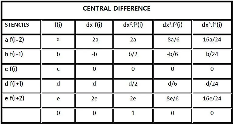
From the table, we have 5 equations and 5 unknown coefficients.

a + b + c + d + e = 0

-2a -b +0 + d + 2e = 0

2a + b/2 + 0 + d/2 + 2e = 1

-8a/6 -b/6 + 0 + d/6 + 8e/6 = 0

16a/24 + b/24 + 0 + d/24 + 16e/24 = 0

The unknown coefficients a, b, c, d, e are resolved using Matlab.

Note: We use the rats(linsolve(A,B)) command here to avoid the errors in rounding off the constants, which arises when we use the inv(A)*B command.

Code:

A = [ 1 1 1 1 1 ; 
      -2 -1 0 1 2 ; 
      4/2 1/2 0 1/2 4/2;
      -8/6 -1/6 0 1/6 8/6; 
      16/24 1/24 0 1/24 16/24];

B = [ 0; 0; 1; 0; 0 ];

Coeffs = rats(linsolve(A,B))

Result:

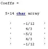
The equation for the Central Difference 2nd order scheme with 4th order accuracy-

2. Skewed Right-Sided Difference scheme

Number of nodes, N = p + q , where p = order of derivative

= 2 + 4 q = order of approximation

= 6

Note: The number of nodes for the Skewed Left-Sided Difference scheme is also 6.

The Taylor Table for Skewed Right-Sided scheme-

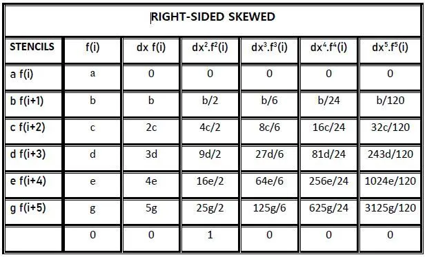
From the table, we have 6 equations and 6 unknown coefficients.

a + b + c + d + e + g = 0

0 + b + 2c + 3d + 4e + 5g = 0

0 + b/2 + 4c/2 + 9d/2 + 16e/2 + 25g/2 = 1

0 + b/6 + 8c/6 + 27d/6 + 64e/6 + 125g/6 = 0

0 + b/24 + 16c/24 + 81d/24 + 256e/24 + 625g/24 = 0

0 + b/120 + 32e/120 + 243d/120 + 1024e/120 + 3125g/120 = 0

The unknown coefficients a, b, c, d, e and g are again resolved in Matlab.

Code:

A = [ 1 1 1 1 1 1; 
      0 1 2 3 4 5;
      0 1/2 2 9/2 8 25/2;
      0 1/6 8/6 27/6 64/6 125/6;
      0 1/24 16/24 81/24 256/24 625/24;
      0 1/120 32/120 243/120 1024/120 3125/120 ];

B = [ 0; 0; 1; 0; 0; 0 ];

Coeffs = rats(linsolve(A,B))

Result:

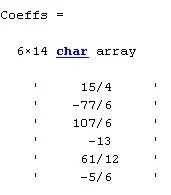
The equation for the Skewed Right-Sided Difference 2nd order scheme with 4th order accuracy-

3. Skewed Left-Sided Difference scheme

The Taylor Table for Skewed Left-Sided scheme-

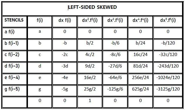
From the table, we have 6 equations and 6 unknown coefficients.

a + b + c + d + e + g = 0

0 - b - 2c - 3d - 4e - 5g = 0

0 + b/2 + 4c/2 + 9d/2 + 16e/2 + 25g/2 = 1

0 - b/6 - 8c/6 - 27d/6 - 64e/6 - 125g/6 = 0

0 + b/24 + 16c/24 + 81d/24 + 256e/24 + 625g/24 = 0

0 - b/120 - 32e/120 - 243d/120 - 1024e/120 - 3125g/120 = 0

Code:

A = [ 1 1 1 1 1 1; 
      0 -1 -2 -3 -4 -5; 
      0 1/2 2 9/2 8 25/2;
      0 -1/6 -8/6 -27/6 -64/6 -125/6;
      0 1/24 16/24 81/24 256/24 625/24;
      0 -1/120 -32/120 -243/120 -1024/120 -3125/120 ]
  
B = [ 0; 0; 1; 0; 0; 0 ]

Coeffs = rats(linsolve(A,B))

Result:

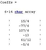
The equation for the Skewed Left-Sided Difference 2nd order scheme with 4th order accuracy-

CODE:

1. Main code

clear all
close all
clc

% Analytical Function = exp(x)*cos(x)
% Analytical derivative = -2*exp(x)*sin(x)

% Parameters

x = pi/3;
dx = linspace(pi/4,pi/400,100);

for i = 1:length(dx)
    
    central_difference_error(i) = Central_Difference_approx(x,dx(i));
    skewed_right_sided_error(i) = Skewed_Right_Sided_approx(x,dx(i));
    skewed_left_sided_error(i) = Skewed_Left_Sided_approx(x,dx(i));
    forward_difference_error(i) = Forward_Difference_approx(x,dx(i));
    backward_difference_error(i) = Backward_Difference_approx(x,dx(i));
  
end

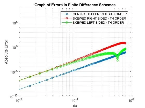
figure(1)

loglog(dx, central_difference_error,'marker','pentagram') 
hold on
loglog(dx, skewed_right_sided_error,'r','marker','hexagram')
hold on
loglog(dx, skewed_left_sided_error,'g','marker','d')
axis([10^(-2) 10^(0) 10^(-10) 10^(8)])
grid on
xlabel('dx')
ylabel('Absolute Error')
title('Graph of Errors in Finite Difference Schemes')
legend('CENTRAL DIFFERENCE 4TH ORDER','SKEWED RIGHT SIDED 4TH ORDER','SKEWED LEFT SIDED 4TH ORDER')

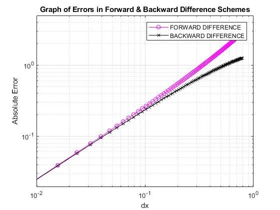
figure(2)
loglog(dx,forward_difference_error,'m','marker','o')
hold on
loglog(dx,backward_difference_error,'k','marker','x')
axis([10^(-2) 10^(0) 0 5])
grid on
xlabel('dx')
ylabel('Absolute Error')
title('Graph of Errors in Forward & Backward Difference Schemes')
legend('FORWARD DIFFERENCE','BACKWARD DIFFERENCE')

2. Function

% Function for Central Difference Approximation

function out = Central_Difference_approx(x,dx)

analytical_derivative = -2*exp(x)*sin(x);

central_difference_derivative = (((-1/12)*exp(x-2*dx)*cos(x-2*dx))+((4/3)*exp(x-dx)*cos(x-dx))+((-5/2)*exp(x)*cos(x))+((4/3)*exp(x+dx)*cos(x+dx))+((-1/12)*exp(x+2*dx)*cos(x+2*dx)))/((dx)^2);

out = abs(central_difference_derivative-analytical_derivative);


% Function for Skewed Right-Sided Approximation

function out = Skewed_Right_Sided_approx(x,dx)

analytical_derivative = -2*exp(x)*sin(x);

skewed_right_sided_derivative = (((15/4)*exp(x)*cos(x))+((-77/6)*exp(x+dx)*cos(x+dx))+((107/6)*exp(x+2*dx)*cos(x+2*dx))+((-13)*exp(x+3*dx)*cos(x+3*dx))+((61/12)*exp(x+4*dx)*cos(x+4*dx))+((-5/6)*exp(x+5*dx)*cos(x+5*dx)))/((dx)^2);

out = abs(skewed_right_sided_derivative-analytical_derivative);


% Function for Skewed Left-Sided Approximation

function out = Skewed_Left_Sided_approx(x,dx)

analytical_derivative = -2*exp(x)*sin(x);

skewed_left_sided_derivative = (((15/4)*exp(x)*cos(x))+((-77/6)*exp(x-dx)*cos(x-dx))+((107/6)*exp(x-2*dx)*cos(x-2*dx))+((-13)*exp(x-3*dx)*cos(x-3*dx))+((61/12)*exp(x-4*dx)*cos(x-4*dx))+((-5/6)*exp(x-5*dx)*cos(x-5*dx)))/((dx)^2);

out = abs(skewed_left_sided_derivative-analytical_derivative);


% Function for Forward Difference Approximation

function out = Forward_Difference_approx(x,dx)

analytical_derivative = exp(x)*(cos(x) - sin(x));

forward_difference_derivative = ((exp(x+dx)*cos(x+dx))-(exp(x)*cos(x)))/(dx);

out = abs(forward_difference_derivative-analytical_derivative);



% Function for Backward Difference Approximation

function out = Backward_Difference_approx(x,dx)

analytical_derivative = exp(x)*(cos(x) - sin(x));

backward_difference_derivative = ((exp(x)*cos(x))-exp(x-dx)*cos(x-dx))/(dx);

out = abs(backward_difference_derivative-analytical_derivative);

RESULTS:

CONCLUSION:

The key findings can be summarized as follows-

• The central difference scheme has the minimum absolute error when compared to the skewed right-sided and left-sided difference schemes which show a somewhat similar trend in terms of the error. However, as the dx (mesh size) decreases, the analysis loses stability and accuracy drastically, resulting in an increase in the absolute errors once the grid size value goes below 10^(-2). This occurs as a result of the rounding off of the errors.

• The order of accuracy of both Forward and backward difference schemes is much lower compared to the finite difference schemes as they are of the first order and utilize information either from the right or left of the central node respectively. These lead to inaccuracy and instability in the numerical analysis, as the grid size increases for the said schemes. The type of analytical function e.g. periodic functions, etc. employed also plays an important factor in the error propagation.

• Central(finite) differences due to their simple anti-symmetric structure and overall accuracy, are very widely used in numerical analysis. However, skewed schemes are more useful in complex geometries e.g. flow over a compressor blade, heat flow over a plate in a particular direction, and around complicated boundary conditions where the central differencing scheme cannot be accurately employed.