Otto Cycle using Piston Kinematics using MATLAB and Python

Aim:- To solve and plot PV-Diagram of an otto cycle considering engine Kinematics.

Objective:-

• To plot an otto cycle.
• Calculate Thermal efficiency.

Theory:-

Thermodynamics is a branch of physics that deals with heat and temperature, and their relation to energy, work, radiation, and properties of matter.

An Otto cycle is an idealized thermodynamic cycle that describes the functioning of a typical spark ignition piston engine.The Otto cycle is a description of what happens to a mass of gas as it is subjected to changes of pressure, temperature, volume, addition of heat, and removal of heat.

Otto cycle Processes and formulas:-

1. Isentropic compression (compression stroke) – The gas (fuel-air mixture) is compressed adiabatically from state 1 to state 2, as the piston moves from bottom dead center to top dead center.
2. Isochoric compression (ignition phase) – In this phase (between state 2 and state 3) there is a constant-volume (the piston is at rest ) heat transfer to the air from an external source while the piston is at rest at top dead center.
3. Isentropic expansion (power stroke) – The gas expands adiabatically from state 3 to state 4, as the piston moves from top dead center to bottom dead center.
4. Isochoric decompression (exhaust stroke) – In this phase the cycle completes by a constant-volume process in which heat is rejected from the air while the piston is at bottom dead center. The working gas pressure drops instantaneously from point 4 to point 1.

Formulas Used :-

• Swept Volume(v_s)- (pi/4)*bore^2*stroke
• Clearance volume(v_c)- v_s/(cr-1)
• Variation of volume inside the cylinder with crank angle-

V=(1+0.5*(cr-1)*(R+1-cosd(theta)-(R^2-sind(theta).^2).^0.5))*v_c

Governing Thermodynamics Equations:-

Thermal efficiency of otto cycle=

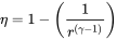
Isentropic process= An adiabatic and reversilbe process.Its equation is

p.v^gamma=constant

Ideal gas equation= p.v/t=constant

Procedure:-

Inputs to our program will be:-

• Bore
• Stroke length
• connecting rod length
• p1,v1
• t3
• commpression ratio(c_r)
• Gamma

CODE IN MATLAB:-

clear all
close all
clc

%Inputs Parameter
gamma=1.4;
t3=2300;

%state variables
p1=102000;
t1=450;

%Engine geometric parameters
bore=0.1;
stroke=0.1;
c_rod=0.15;
cr=12;

%calculate the swwept volume and clearence volume
v_s=(pi/4)*bore^2*stroke;
v_c=v_s/(cr-1);

v1=v_s+v_c;
v2=v_c;

v_com=engine_kinematics(bore,stroke,c_rod,cr,0,180);
const=p1*v1^gamma;
p_com=const./v_com.^gamma;


%state variables at state point 2
%Now, p2v2^gamma=p1v1^gamma then
p2=p1*cr^gamma;

%And p1v1/t1=p2v2/t2 therefore
t2=p2*v2*t1/(p1*v1);

%state variables at state point 3
v3=v2;

%p3v3/t3=p2v2/t2 therefore
p3=p2*t3/t2;

%state variables at state point 4
v4=v1;

%p3v3^gamma=p4v4^gamma then
p4=p3*(v3/v4)^gamma;

v_exp=engine_kinematics(bore,stroke,c_rod,cr,360,540);
const1=p3*v3^gamma;
p_exp=const1./v_exp.^gamma;

figure(1)
hold on
plot(v1,p1,'*','color','r')
plot(v_com,p_com,'r')
plot(v2,p2,'*','color','r')
plot([v2 v3],[p2 p3],'r')
plot(v3,p3,'*','color','r')
plot(v_exp,p_exp,'r')
plot(v4,p4,'*','color','r')
plot([v4 v1],[p4 p1],'r')

xlabel('Volume(m^3)')
ylabel('Pressure(Pa)')
title('P-V Diagram of an Otto cycle')

%Thermal Efficiency of an otto cycle
E=(1-(1/cr^(gamma-1)))*100;
fprintf('Thermal Efficiency of an otto cycle is:- %f',E);

Code to calculate the Function using piston kinematics:-

function [V]=engine_kinematics(bore,stroke,c_rod,cr,start_crank,end_crank)

a=stroke/2;
R=c_rod/a;

v_s=(pi/4)*bore^2*stroke;
v_c=v_s/(cr-1);

theta=linspace(start_crank,end_crank,100);

V=(1+0.5*(cr-1)*(R+1-cosd(theta)-(R^2-sind(theta).^2).^0.5))*v_c;

end

Steps:-

• Firstly, Inputs are provided in our Editor and swept volume and clearance volume is calculated using above formula and then v_1 and v_2 are calculated using swept volume and clearance volume.
• Then we will create an function to claculate the Variation of volume inside the cylinder with diferent crank angle from 1 to 180 degrees using input to the function and assign it to v_com.
• Then we will calculate state variable at state point 2 , 3 and 4 using isentropic equation and ideal gas equation and then at state pont 4 we will assign engine_kinematics in the v_exp.
• Then we will plot the state point and the lines between these state points.
• Then we will calculate thermal efficiency of an otto cycle using above mentioned formula.

Error faced during execution in Matlab:-

We will find an error that the plotting of state point have disconnenct line.

Correction:-

It can be corrected by the giving full input to the plotting plot([v1 v2 v3 v4 v1]),[p1 p2 p3 p4]) by completing full loop.

But the above plot of PV Diagram of an otto cycle is wrong which can be corrected by using engine_kinematic function which follow the piston kinematic to get the correct result.

CODE IN PYTHON :-

# Otto cycle simulation

import math
import matplotlib.pyplot as plt

def engine_kinematics(bore, stroke, c_rod, c_r, start, end):
    

    # Geometric Parameters

    a = stroke/2
    R = c_rod/a


    # Volume parameters
    v_s = (math.pi/4)*pow(bore,2)*stroke
    v_c = v_s/(c_r-1)


    sc = math.radians(start)
    ec = math.radians(end)
    
    n = 50
    d = (ec -sc)/(n-1)
    
    V =[]
    
    for i in range(0,n):
        theta = sc + i*d
        term1 = 0.5*(c_r-1)
        term2 = R + 1 - math.cos(theta)
        term3 = pow(R,2) - pow(math.sin(theta),2)
        term3 = pow(term3, 0.5)
        V.append((1 + term1*(term2-term3))*v_c)
        
    return V

#Inputs
gamma = 1.4
t3 = 2300
p1 = 102000
t1 = 450

# Geometric parameters
bore = 0.1
stroke = 0.1
c_rod = 0.15
c_r = 12

# Calculate swept volume and clearance volume
v_s = (math.pi/4)*pow(bore,2)*stroke
v_c = v_s/(c_r-1)

v1 = v_s + v_c

#state point 2
v2 = v_c

# p2v2^gamma = p1v1^gamma
p2 = p1*pow(c_r,gamma)

# And p1v1/t1=p2v2/t2 then
t2 = p2*v2*t1/(p1*v1)

V_comm = engine_kinematics(bore, stroke, c_rod, c_r, 180, 0)

constant = p1*pow(v1,gamma)
P_comm = []

for v in V_comm:
    P_comm.append(constant/pow(v,gamma))
    

# State variables at state point 3
v3 = v2

#p3v3/t3 = p2v2/t2 then
p3 = p2*t3/t2


V_exp = engine_kinematics(bore, stroke, c_rod, c_r, 0, 180)

constant = p3*pow(v3,gamma)
P_exp = []

for v in V_exp:
    P_exp.append(constant/pow(v,gamma))
    
    
# State variables at state point 4
v4 = v1

# p3v3^gamma = p4v4^gamma
p4 = p3*pow(v3,gamma)/pow(v4,gamma)




plt.plot([v2,v3],[p2,p3])
plt.plot(V_comm,P_comm)
plt.plot(V_exp,P_exp)
plt.plot([v4,v1],[p4,p1])

plt.xlabel('Volume(m^3)')
plt.ylabel('Pressure(Pa)')
plt.title('P-V Daigram of an Otto Cycle')
plt.show()

#Thermal Efficiency of an otto cycle
E = (1-(1/pow(c_r,(gamma-1))))*100
print('Thermal Efficiency of an otto cycle is :- ',E)     

Steps:-

• Firstly, we will import math and matplotlib library in python.
• Then we will create an engine_kinematics function considering piston kinematics and inputs all the parameters then we will create start crank angle and end crank angle to have range of crank angle which can be created using loop in which we assign the volume for different crank angle to append all values of volume to an empty array of volume then we will provide this each volume values to our function by using return command.
• Now we will end this function and at the new line we will input parameters and geometric paramaters and then we will find the state variables of the all the state points.
• Now in the commpression and expansion state point we will call this functions and find pressure commpression and expansion using loop.
• Then we will plot our all state variables and Find Thermal efficiency of an otto cycle.

Error faced during execution:-

Error faced due to invalid use of syntax in the efficiency formula by not creating bracket.

RESULTS:-

Plot of an Otto cycle using Matlab:-

Thermal Efficiency of an otto cycle:- 62.98%