Simulation of a 1D Super-sonic nozzle flow simulation using MacCormack Method in MATLAB
OBJECTIVES:
- Derive both the conservation and non-conservation forms of the governing equations and solve them using MacCormack's technique.
- Steady-state distribution of primitive variables inside the nozzle.
- Time-wise variation of the primitive variables.
- Variation of Mass flow rate distribution inside the nozzle at different time steps during the time-marching process.
- Comparison of Normalized mass flow rate distributions of both forms.
- To perform a grid independence test on both solutions.
1. INTRODUCTION
A steady, isentropic (reversible and adiabatic) flow through a convergent-divergent nozzle is considered. The flow at the inlet to the nozzle comes from a reservoir where the pressure and temperature are denoted by `p_o` and `T_o` respectively. The cross-sectional area of the reservoir is large(theoretically, `Ararrinfty`), and hence the velocity is very small (`Vrarr0`). Thus `p_o` and `T_o` are the stagnation values, or total pressure and temperature respectively. The flow expands isentropically to supersonic speeds at the nozzle exit, where the exit pressure, temperature, velocity, and Mach number are denoted by `p_e`, `T_e`, `V_e`, and `M_e`, respectively. The flow is locally subsonic in the convergent section of the nozzle, sonic at the throat (minimum area), and supersonic at the divergent section.
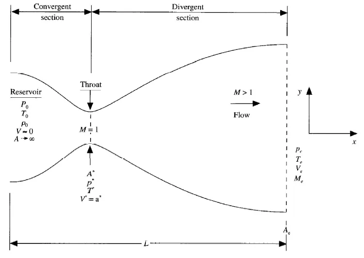
Fig.1: subsonic-supersonic nozzle flow
The sonic flow (M=1) at the throat means that the local velocity is equal to the local speed of sound. At the throat, `V=V^**=a^**`. Similarly, the other sonic flow values are `p^**`, `T^**`, and `A^**`. It is assumed that the flow properties vary only with x, such a flow is defined as quasi-one-dimensional flow.
The governing continuity, momentum, and energy equations for this flow can be expressed as
Continuity: `rho_1V_1A_1 = rho_2V_2A_2` `rarr(1)`
Momentum: `rho_1A_1+rho_1V_1^2A_1+int_(A_1)^(A_2)p.dA=p_2A_2+rho_2V_2^2A_2` `rarr(2)`
Energy: `h_1+V_1^2/2=h_2+V_2^2/2` `rarr(3)`
Subscripts 1 and 2 denote different locations along the nozzle. Also,
`p=rhoRT` (perfect gas equation) `rarr(4)`
`h=c_pT` `rarr(5)`
The Mach number variation through the nozzle is governed exclusively by the ration `A/A^**` through the relation
`(A/A^**)^2=1/M^2[2/(gamma+1)(1+(gamma-1)/2M^2)]^((gamma+1)/(gamma-1))` `rarr(6)`
where `gamma`= ratio of specific heats = `c_p/c_v`. Also, the variation of pressure, density, and temperature as a function of Mach number (and thus as a function of `A/A^**`, thus `x`) is given respectively by
`p/p_o=(1+(gamma-1)/2M^2)^(-gamma/(gamma-1))` `rarr(7)`
`rho/rho_o=(1+(gamma-1)/2M^2)^(-1/(gamma-1))` `rarr(8)`
`T/T_o=(1+(gamma-1)/2M^2)^(-1)` `rarr(9)`
The force required for the nozzle to accelerate through the nozzle is provided by the pressure ratio across the nozzle `p_o/p_e`.
2. Set-up
The three echelons of equations are as follows:
- The governing equations will be written in terms of PDEs suitable for the time-marching solution of the quasi-one-dimensional flow
- The finite-difference expressions pertaining to MacCormack's technique as applied to this problem will be set up.
- The other details for the numerical solution such as the calculation of the time step and the treatment of boundary conditions will be formulated.
2.1 Governing Flow Equations in non-conservation form
Since the flow is assumed to be quasi-one-dimensional, the governing partial differential equations for inviscid flow (the Euler eqns) cannot be applied here. The integral form of the governing eqns. are applied to a control volume consistent with the quasi-one-dimensional assumption.
Continuity: `(delta(rhoA))/(deltat)+rhoA(deltaV)/(deltax)+rhoV(deltaA)/(deltax)+VA(deltarho)/(deltax)=0` `rarr(10)`
Momentum: `rho(deltaV)/(deltat)+rhoV(deltaV)/(deltax) = -R (rho(deltaT)/(deltax)+T(deltarho)/(deltax))` `rarr(11)`
Energy: `rhoc_v(deltaT)/(deltat)+rhoVc_v(deltaT)/(deltax)= -rhoRT[(deltaV)/(deltax)+V(delta(ln A))/(deltax)]` `rarr(12)`
These are written as dimensional variables, and for nozzle flows, the flow field variables are frequently expressed in terms of non-dimensional variables, where the flow variables are referenced to their reservoir values. The non-dimensional variables `p/p_o`, `rho/(rho_o)` and `T/T_o` vary between 0 and 1. We define these terms below, where the prime denotes a dimensionless variable.
Non-dimensional temperature: `T' = T/T_o`
Non-dimensional density: `rho' = rho/rho_o`
Non-dimensional length: `x' = x/L`
Non-dimensional velocity: `V'=V/a_o`, where `a_o`=speed of sound in the reservoir = `sqrt(gammaRT_o)`
Non-dimensional time: `t'=t/(L/a_o`
Non-dimensional area: `A'=A/(A^**)`
Introducing these variables in eqns. `10`, `11` and `12`, we get the form of the governing eqns. most appropriate for the time-marching solution of quasi-one-dimensional flow.
Continuity: `(deltarho^')/(deltat^')=-rho^'(deltaV^')/(deltax^')+rho^'V^'(delta(ln A^'))/(deltax^')-V^'(deltarho^')/(deltax^')` `rarr(13)`
Momentum: `(deltaV^')/(deltat^')=-V(deltaV^')/(deltax^')-1/gamma ((deltaT^')/(deltax^')+T^'/rho^'(deltarho^')/(deltax^'))` `rarr(14)`
Energy: `(deltaT^')/(deltat^')=-V^'(deltaT^')/(deltax^')-(gamma-1)T^'[(deltaV^')/(deltax^')+V^'(delta(ln A^'))/(deltax^')]` `rarr(15)`
2.2 Finite Difference Eqns. using MacCormack's method
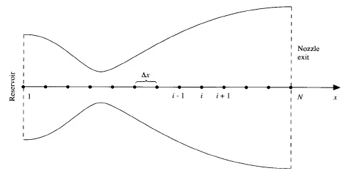
Fig.2: Grid point distribution along the nozzle
The next step is setting up of the finite-difference expressions using MacCormack's explicit technique for the numerical solution of eqns. `13`, `14` and `15`.The x-axis is divided along the nozzle into a number of grid points (see Fig.2). The first grid point 1 is assumed to be in the reservoir. The points are distributed evenly along the x-axis and `Deltax` denotes the spacing between the grid points. N denotes the last point at the nozzle exit. This technique is a predictor-corrector method. Henceforth, all variables are non-dimensional variables and prime is dropped.
1. Predictor-step
The spatial derivatives are set up as forward differences. From eqns. 13, 14 and 15
`((deltarho)/(deltat))_i^t=-rho_i^t(V_(i+1)^t-V_i^t)/(Deltax)-rho_i^tV_i^t(ln A_(i+1)-ln A_i)/(Deltax)-V_i^t(rho_(i+1)^t-rho_i^t)/(Deltax)` `(rarr16)`
`((deltaV)/(deltat))_i^t=-V_i^t(V_(i+1)^t-V_i^t)/(Deltax)-1/gamma((T_(i+1)^t-T_i^t)/(Deltax)+T_i^t/rho_i^t(rho_(i+1)^t-rho_i^t)/(Deltax))` `(rarr17)`
`((deltaT)/(deltat))_i^t=-V_i^t(T_(i+1)^t-T_i^t)/(Deltax)-(gamma-1)T_i^t((V_(i+1)^t-V_i^t)/(Deltax)+V_i^t(ln A_(i+1)-ln A_i)/(Deltax))` `(rarr18)`
Predicted values of `rho`, `V`, and `T` are obtained from
`bar rho_i^(t+Deltat)=rho_i^t+((deltarho)/(deltat))_i^tDeltat` `(rarr19)`
`bar V_i^(t+Deltat)=V_i^t+((deltaV)/(deltat))_i^tDeltat` `(rarr20)`
`bar T_i^(t+Deltat)=T_i^t+((deltaT)/(deltat))_i^tDeltat` `(rarr21)`
2. Corrector Step
The spatial derivatives are replaced here with backward differences, using the predicted quantities.
`(bar(deltarho)/(deltat))_i^(t+Deltat)=-barrho_i^(t+Deltat)(barV_i^(t+Deltat)-barV_(i-1)^(t+Deltat))/(Deltax)-barrho_i^(t+Deltat)barV_i^(t+Deltat)(ln A_i-ln A_(i-1))/(Deltax)-barV_i^(t+Deltat)(barrho_i^(t+Deltat)-barrho_(i-1)^(t+Deltat))/(Deltax)` `(rarr22)`
`(bar(deltaV)/(deltat))_i^(t+Deltat)=-barV_i^(t+Deltat)(barV_i^(t+Deltat)-barV_(i-1)^(t+Deltat))/(Deltax)-1/gamma((barT_i^(t+Deltat)-barT_(i-1)^(t+Deltat))/(Deltax)+barT_i^(t+Deltat)/barrho_i^(t+Deltat)(barrho_i^(t+Deltat)-barrho_(i-1)^(t+Deltat))/(Deltax))` `(rarr23)`
`(bar(deltaT)/(deltat))_i^(t+Deltat)=-barV_i^(t+Deltat)(barT_i^(t+Deltat)-barT_(i-1)^(t+Deltat))/(Deltax)-(gamma-1)barT_i^(t+Deltat)((barV_i^(t+Deltat)-barV_(i-1)^(t+Deltat))/(Deltax)+barV_i^t(ln A_i-ln A_(i-1))/(Deltax))` `(rarr24)`
The average time derivatives are given by
`((deltarho)/(deltat))_(av)=0.5[((deltarho)/(deltat))_i^t + (bar(deltarho)/(deltat))_i^(t+Deltat)]` `(rarr25)`
`((deltaV)/(deltat))_(av)=0.5[((deltaV)/(deltat))_i^t + (bar(deltaV)/(deltat))_i^(t+Deltat)]` `(rarr26)`
`((deltaT)/(deltat))_(av)=0.5[((deltaT)/(deltat))_i^t + (bar(deltaT)/(deltat))_i^(t+Deltat)]` `(rarr27)`
Finally, the corrected values of the flow-field variables at time `t+Deltat`
`rho_i^(t+Deltat)=rho_i^t+ ((deltarho)/(deltat))_(av)Deltat` `(rarr28)`
`V_i^(t+Deltat)=V_i^t+ ((deltaV)/(deltat))_(av)Deltat` `(rarr29)`
`T_i^(t+Deltat)=T_i^t+ ((deltaT)/(deltat))_(av)Deltat` `(rarr30)`
2.3 Time-Step and Boundary Conditions
2.3.1 Calculation of Time-Step:
The governing system of equations, Eqns. 13, to 15, is hyperbolic w.r.t. time. The stability constraint for this system is
`Deltat = C(Deltax)/(a+V)` `(rarr31)`
Eqn. 31 is the Courant-Friedrichs_Lowry (CFL) criterion for a one-dimensional flow, where C is the Courant Number, `V` is the local flow velocity at a point in the flow, and `a` is the local speed of sound. Eqn. `31` along with `C<=1`, states that `Deltat` must be less than, or equal to, the time it takes a sound wave to move from one point to the next.
In the implementation of the time-marching solution, it is chosen to calculate `(Deltat)_i^t`at all the grid points, `i=1` to `i=N`, and then the minimum value is used in the eqns.
`Deltat` = minimum `(Deltat_1^t,Deltat_2^t,........Deltat_N^t)`
The flow-field variables at all the grid points at time `t+Deltat` all correspond to the same physical time. Thus, the solution gives a time-accurate solution of the actual transient flow field, consistent with the unsteady continuity, momentum, and energy equations.
2.3.2 Boundary Conditions:
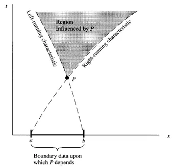
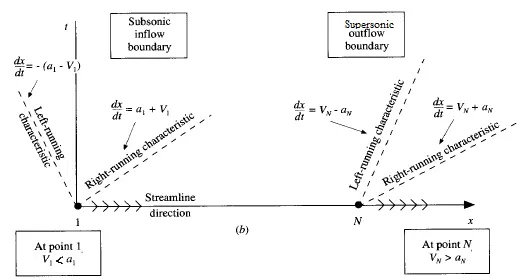
Another important aspect of the numerical solution is that of boundary conditions. Unsteady, inviscid flow is governed by hyperbolic equations. Therefore, two characteristic lines exist through any point in the xt-plane (fig below). Physically, these represent infinitely weak Mach waves that are propagating upstream and downstream at the speed of sound `a` (Fig below).
(a)
(b)
Fig.3: (a) Domain for soln of hyperbolic equations, (b) State of boundary conditions
The method of characteristics tells us that at a boundary, if one characteristic propagates into the domain, then the value of one dependent flow-field variable must be specifies at the boundary. And if one characteristic line propagates out of the domain, then the value of another flow-field variable must be allowed to float at the boundary, i.e., it must be calculated in steps of time as a function of the timewise solution of the flow field. Thus, at the subsonic inflow boundary, two dependent flow-field variables must be stipulated and one other variable must be allowed to float. At the supersonic outflow boundary, both the characteristics propagate out of the domain. So, all variables are allowed to float at this boundary.
- Subsonic inflow boundary (point 1)
Velocity `V_1` is allowed to float as the mass flow through the nozzle must be allowed to adjust to the proper steady state. `V_1` changes with time and is calculated from the flow-field solution over the internal points (points 2 through `N-1` in `Fig.2`). Linear extrapolation is used to calculate `V_1` from points 2 and 3.
Slope = `(V_3-V_2)/(Deltax)`
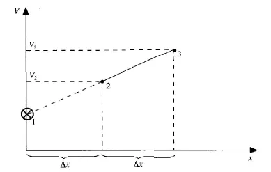
Fig.4: Linear extrapolation
`V_1 =V_2-(V_3-V_2)/(Deltax)Deltax`
`rArr V_1=2V_2-2V_3)`
- Supersonic outflow boundary (point N)
All flow-field variables are floated.
`V_N=2V_(N-1)-V_(N-2))`
`rho_N=2rho_(N-1)-rho_(N-2))`
`T_N=2T_(N-1)-T_(N-2))`
- Nozzle shape and initial conditions
The nozzle shape, `AequivA(x)` is specified and held fixed, independent of time.
`A=1+2.2(x-1.5)^2 0<=x<=3`
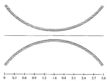
Fig.5: Distance along nozzle
The initial conditions at t = 0 are assumed considering `rho` and `T` decreases and `V` increases as the flow expands through the nozzle.
`rho = 1 - 0.3146x`
`T = 1 - 0.2314x`
`V = (0.1+1.09)T^(1/2)`
3.1 Governing Flow Equations in conservation form
Equations `32,33`, and `34` are the non-dimensional conservation form of the continuity, momentum, and energy equations for quasi-1D flow.
`(del(rho'A'))/(delt') + (del(rho'A'V'))/(delx')=0`, `rarr(32)`
`(del(rho'A'V'))/(delt')+(del[rho'A'V'+(1/gamma)rho'A'])/(delx')=1/gamma p'(del(A'))/(delt') `, `rarr(33)`
`(del[rho'A'((e')/(gamma-1)+gamma/2(V')^2)])/(delt')+ (del[rho'A'V'((e')/(gamma-1)+gamma/2(V')^2)+rho'A'V'])/(delx')=0` `rarr(34)`
The generic form of the governing equations for unsteady, 3D flow is given as
`(delU)/(delt)+(delF)/(delx)+(delG)/(dely)+(delH)/(delz)=J` 'rarr(35)'
if `U,F,G,H`,and `J`are column vectors given by
`U=((rho),(rhou),(rhov),(rhow),(rho(e+V^2/2)))` `rarr(36)`
`F=((rhou),(rhou^2+p-tau_(x x)),(rhovu-tau_(xy)),(rhowu-tau_(xz)),(rho(e+V^2/2)u+pu-k(delT)/(delx)-utau_(x x)-vtau_(xy)-wtau_(xz)))` `rarr(37)`
`G=((rhov),(rhouv-tau_(yx)),(rhov^2+p-tau_(y y)),(rhowv-tau_(yz)),(rho(e+V^2/2)v+pv-k(delT)/(dely)-utau_(y x)-vtau_(yy)-wtau_(yz)))` `rarr(38)`
`H=((rhow),(rhouw-tau_(zx)),(rhovw-tau_(zy)),(rhow^2+p-tau_(z z)),(rho(e+V^2/2)w+prhow-k(delT)/(delz)-utau_(zx)-vtau_(zy)-wtau_(z z)))` `rarr(39)`
`J=((0),(rhof_x),(rhof_y),(rhof_z),(rho(uf_x+vf_y+wf_z)+rhodotq))` `rarr(40)`
The column vectors `F`,`G`,and `H` are called the flux terms (or flux vectors) and `J` is the source vector. The column vector `U` is called the solution vector.
The equations for quasi-1D flow can also be expressed in a similar generic form. The elements of the vectors `U`,`F`, and `J` are as follows.
`U_1=rho'A'`
`U_2=rho'A'V'`
`U_3=rho'A'((e')/(gamma-1)+gamma/2(V')^2))`
`F_1=rho'A'V'`
`F_2=rho'A'(V')^2+1/gammap'A'`
`F_3=rho'A'V'((e')/(gamma-1)+gamma/2(V')^2))+p'A'V'`
`J_2=1/gammap'(delA')/(delx')`
With these elements eqns `32,`33`, and `34` can be written as
`(delU_1)/(delt')=-(delF_1)/(delx')` `rarr(41)`
`(delU_2)/(delt')=-(delF_2)/(delx')+J_2` `rarr(42)`
`(delU_3)/(delt')=-(delF_3)/(delx')` `rarr(43)`
The eqns `41`, `42`, and `43` represent the continuity, momentum, and energy eqn. for quasi-1D flow in conservation. These equations are subsequently solved using MacCormack's technique.
The dependent variables are not the primitive variables in the conservation form. The elements `U_1`, `U_2`, and `U_3` are decoded to obtain the primitive variables (rho, V, T, p, etc.).
`rho'=U_1/A'` `rarr(44.a)`
`V'=U_2/U_1` `rarr(44.b)`
`T'=e'=(gamma-1)((U_3)/(U_2)-gamma/2(V')^2)` `rarr(44.c)`
`p'=rho'T'` `rarr(44.d)`
3.2 Set-up
It is best to use `F_1`,`F_2`,and `F_3` directly in terms of the dependent variables `U_1`,`U_2`,and `U_3` and avoid use of the primitive variables. Otherwise, numerical difficulties arise.
Therefore,
`F_1=U_2` `rarr(45)`
`F_2 = (U_2^2)/(U_1)+(gamma-1)/gamma(U_3-gamma/2(U_2^2)/(U_1))` `rarr(46)`
`F_3= gamma(U_2U_3)/(U_1)-(gamma(gamma-1))/2(U_2^3)/(U_1^2)` `rarr(47)`
The source term`J_2`
`J_2=1/gammap'(delA')/(delx')` `rarr(48)`
3.3 Boundary & Initial condtions
- Subsonic inflow boundary (point 1)
`rho' = 1`, `T'=1`
`U_(1(i=1))=(rho'A')_(i=1)= A'_(i=1)`= fixed value
`U_(2(i=1))=2U_(2(i=2))-U_(2(i=3)) `
`U_3 = U_1((T')/(gamma-1)+gamma/2(V')^2)`
- Supersonic outflow boundary (point N)
`(U_1)_N=2(U_1)_(N-1)-(U_1)_(N-2) `
`(U_2)_N=2(U_2)_(N-1)-(U_2)_(N-2) `
`(U_3)_N=2(U_3)_(N-1)-(U_3)_(N-2) `
Initial Conditions
`obrace((rho'=1.0),(T'=1.0))^("for 0<=x'<=0.5")`, `obrace((rho'=1.0-0.366(x'-0.5)),(T'=1.0-0.167(x'-0.5)))^("for 0.5<=x'<=1.5")`, `obrace((rho'=0.634-0.3879(x'-1.5)),(T'=0.833-0.3507(x'-1.5)))^("for 1.5<=x'<=3")`
For the initial conditions, a constant mass flow through the nozzle is assumed.
`V'=U_2/(rho'A')=0.59/(rho'A')`
CODE:
1. Main code
% Main Code
clear all
close all
clc
% Inputs
L=3;
n=31;
x=linspace(0,L,n);
a = 1+2.2*(x-1.5).^2;
nt=1400;

[rho_nc,temp_nc,v_nc,M_nc,p_nc,rho_th_nc,M_th_nc,p_th_nc,temp_th_nc,rho_res_nc,v_res_nc,temp_res_nc,m_nc]=Non_Conservation_function(n,L);
[rho_c,temp_c,M_c,p_c,v_c,rho_th_c,M_th_c,p_th_c,temp_th_c,u1_res_c,u2_res_c,u3_res_c,m_c]=Conservation_function(n,L);

% Steady-state distribution of primitive variables
figure(1)
subplot(4,1,1)
plot(x, M_nc, x,M_c,'*')
axis([0 3 0 4])
ylabel('Mach No.')
xticks([0 0.5 1 1.5 2 2.5 3])
legend('Non-conservation form','Conservation form', 'Location','northwest')
hold on
title(sprintf('Steady-state distribution of primitive variables '));

subplot(4,1,2)
plot(x,p_nc, x,p_c,'*')
ylabel('pressure')
xticks([0 0.5 1 1.5 2 2.5 3])
legend('Non-conservation form','Conservation form', 'Location','northwest')
hold on

subplot(4,1,3)
plot(x,rho_nc, x, rho_c,'*')
ylabel('density')
xticks([0 0.5 1 1.5 2 2.5 3])
legend('Non-conservation form','Conservation form', 'Location','northwest')
hold on

subplot(4,1,4)
plot(x,temp_nc, x, temp_c, '*')
xlabel('Length of the nozzle')
ylabel('Temp')
xticks([0 0.5 1 1.5 2 2.5 3])
legend('Non-conservation form','Conservation form', 'Location','northwest')

% Timewise variation of primitive variables
figure(2)
subplot(4,1,1)
plot(M_th_nc)
hold on
plot(M_th_c)
title(sprintf('Time-wise variation of primitive variables at Throat n'))
ylabel('Mach no.')
legend('Non-conservation form','Conservation form')
hold on

subplot(4,1,2)
plot(p_th_nc)
hold on
plot(p_th_c)
ylabel('Pressure')
legend('Non-conservation form','Conservation form')
hold on

subplot(4,1,3)
plot(rho_th_nc)
hold on
plot(rho_th_c)
ylabel('Density')
legend('Non-conservation form','Conservation form')
hold on

subplot(4,1,4)
plot(temp_th_nc)
hold on
plot(temp_th_c)
xlabel('Number of time-steps');
ylabel('Temp');
legend('Non-conservation form','Conservation form')

% Mass flow rate comparison
figure(5)
plot(x,m_nc,'-o')
hold on
plot(x,m_c,'-o')
xlabel('Distance through nozzle');
ylabel('Mass flow rate');
title(sprintf('Comparison of the steady-state mass flow variations'))
legend('Non-conservation form','Conservation form')

% Grid Independence Test
figure(6)
labels = {'Non-conservation form','Conseravation form','Analytical results'};
y_a = [M_th_nc(1400) M_th_c(1400) 1; p_th_nc(1400) p_th_c(1400) 0.528; rho_th_nc(1400) rho_th_c(1400) 0.634; temp_th_nc(1400) temp_th_c(1400) 0.833];
b = bar(y_a);
legend(labels,'location','northoutside','Orientation','Vertical')
xticklabels({'Mach no.','Pressure','Density','Temperature'});
axis auto
title('For 61 grid points') % Change 'n' to 61 grid points and check for grid independence
a_1 = (1:size(y_a,1)).';
x_ax = [a_1-0.25 a_1 a_1+0.25];
for k = 1:size(y_a,1)
    for m = 1:size(y_a,2)
        text(x_ax(k,m),y_a(k,m),num2str(y_a(k,m),'%0.2f'),'HorizontalAlignment','center','VerticalAlignment','bottom')
    end
end

% Residuals
figure(7)
subplot(2,1,1)
plot(linspace(1,nt,nt),v_res_nc);
hold on
plot(linspace(1,nt,nt),rho_res_nc,'g');
hold on
plot(linspace(1,nt,nt),temp_res_nc,'k');
grid on
ylabel('Residues of primitive variables');
legend('Velocity','Density','Temp');
title('Residual plot for non-conservation form');

subplot(2,1,2)
plot(linspace(1,nt,nt),u1_res_c);
hold on
plot(linspace(1,nt,nt),u2_res_c,'g');
hold on
plot(linspace(1,nt,nt),u3_res_c,'k');
grid on
legend('Solution vector u1','Solution vector u2','Solution vector u3');
ylabel('Residues of solution vector');
title('Residual plot for conservation form');
1.1 Function for NC form
% Function for Non-conservation form

function[rho_nc,temp_nc,v_nc,M_nc,p_nc,rho_th_nc,M_th_nc,p_th_nc,temp_th_nc,rho_res_nc,v_res_nc,temp_res_nc,m_nc]=Non_Conservation_function(n,L);

% Inputs
L=3;
n=31;
x=linspace(0,L,n);
dx = x(2)-x(1);
a = 1+2.2*(x-1.5).^2;
pos = find(a==min(a));
gamma = 1.4;
cfl =0.5;

% Number of iterations
nt=1400;

% Initial profiles
rho_nc = 1-0.3146*x;
temp_nc = 1-0.2134*x;
v_nc = (0.1+1.09*x).*temp_nc.^0.5;
M_nc = v_nc./sqrt(temp_nc);
p_nc = rho_nc.*temp_nc;
a = 1+2.2*(x-1.5).^2;
pos = find(a==min(a));
gamma = 1.4;
cfl =0.5;
%total_time =0;

% Outer time loop
for k = 1:nt

    rho_old = rho_nc;
    temp_old = temp_nc;
    v_old = v_nc;

    % Time Step calculation based on Courant number
    dt = min(cfl.*(dx./(sqrt(temp_nc)+v_nc)));
    %total_time = total_time + dt;
    % Predictor step (Forward-differenecing)
    for j = 2:n-1
        dv_dx = (v_nc(j+1)-v_nc(j))/dx;
        dloga_dx = (log(a(j+1))-log(a(j)))/dx;
        drho_dx = (rho_nc(j+1)-rho_nc(j))/dx;
        dtemp_dx = (temp_nc(j+1)-temp_nc(j))/dx;

        % Continuity eqn
        drho_dt_p(j) = -rho_nc(j)*dv_dx - rho_nc(j)*v_nc(j)*dloga_dx - v_nc(j)*drho_dx;

        % Momentum eqn
        dv_dt_p(j) = -v_nc(j)*dv_dx -(1/gamma)*(dtemp_dx+(temp_nc(j)/rho_nc(j))*drho_dx);

        % Energy eqn
        dtemp_dt_p(j) = -v_nc(j)*dtemp_dx - (gamma-1)*temp_nc(j)*(dv_dx + v_nc(j)*dloga_dx);

        % Solution update
        rho_nc(j) = rho_nc(j) + drho_dt_p(j)*dt;
        v_nc(j) = v_nc(j) + dv_dt_p(j)*dt;
        temp_nc(j) = temp_nc(j) + dtemp_dt_p(j)*dt;


    end

    % Corrector step (Backward-differenecing)
    for j = 2:n-1
        dv_dx = (v_nc(j)-v_nc(j-1))/dx;
        dloga_dx = (log(a(j))-log(a(j-1)))/dx;
        drho_dx = (rho_nc(j)-rho_nc(j-1))/dx;
        dtemp_dx = (temp_nc(j)-temp_nc(j-1))/dx;

        % Continuity eqn
        drho_dt_c(j) = -rho_nc(j)*dv_dx - rho_nc(j)*v_nc(j)*dloga_dx - v_nc(j)*drho_dx;

        % Momentum eqn
        dv_dt_c(j) = -v_nc(j)*dv_dx -(1/gamma)*(dtemp_dx+(temp_nc(j)/rho_nc(j))*drho_dx);

        % Energy eqn
        dtemp_dt_c(j) = -v_nc(j)*dtemp_dx - (gamma-1)*temp_nc(j)*(dv_dx + v_nc(j)*dloga_dx);

    end

    % Compute Avg. time derivative

    drho_dt = 0.5*(drho_dt_p + drho_dt_c);
    dv_dt = 0.5*(dv_dt_p + dv_dt_c);
    dtemp_dt =0.5*(dtemp_dt_p + dtemp_dt_c);


    % Final Soln update
    for i = 2:n-1
        rho_nc(i) = rho_old(i) + drho_dt(i)*dt;
        v_nc(i) = v_old(i) + dv_dt(i)*dt;
        temp_nc(i) = temp_old(i) + dtemp_dt(i)*dt;
        p_nc(i) = rho_nc(i)*temp_nc(i);
        M_nc(i)= v_nc(i)/sqrt(temp_nc(i));
    end

    % Applying boundary conditions
    % Inlet
    v_nc(1) = 2*v_nc(2) - v_nc(3);
    % Outlet
    v_nc(n) = 2*v_nc(n-1) - v_nc(n-2);
    rho_nc(n) = 2*rho_nc(n-1) - rho_nc(n-2);
    temp_nc(n) = 2*temp_nc(n-1) - temp_nc(n-2);

    % Primitive variables at Throat (grid point 16)
    rho_th_nc(k)=rho_nc(pos);
    M_th_nc(k) =M_nc(pos);
    p_th_nc(k) = p_nc(pos);
    temp_th_nc(k) =temp_nc(pos);

    % Residues at throat
    rho_res_nc(k)= drho_dt(pos)*dt;
    v_res_nc(k)= dv_dt(pos)*dt;
    temp_res_nc(k)= dtemp_dt(pos)*dt;

    % Mass flow rate
    m_nc = rho_nc.*a.*v_nc;

    figure(3)
    hold on

    if (k==50)
        plot(x,m_nc,'linewidth',1.5,displayName='time step = 50')
    end
    if (k==100)
        plot(x,m_nc,'linewidth',1.5,displayName='time step = 100')
    end
    if (k==150)
        plot(x,m_nc,'linewidth',1.5,displayName='time step = 150')
    end
    if (k==200)
        plot(x,m_nc,'linewidth',1.5, displayName='time step = 200')
    end
    if (k==700)
        plot(x,m_nc,'linewidth',1.5, displayName='time step = 700')
    end
    legend
    title(sprintf('Variation of mass-flow rate distribution at different time-steps  n Non-conservation form'));
    xlabel('Length of the nozzle');
    ylabel('Mass flow rate');

end
1.2 Function for Conservation form
% Function for Conservation Form

function[rho_c,temp_c,M_c,p_c,v_c,rho_th_c,M_th_c,p_th_c,temp_th_c,u1_res_c,u2_res_c,u3_res_c,m_c]=Conservation_function(n,L);

% Inputs
L=3;
n=31;
x=linspace(0,L,n);
dx = x(2)-x(1);
a = 1+2.2*(x-1.5).^2;
pos = find(a==min(a));
gamma = 1.4;
cfl =0.5;

% Number of iterations
nt=1400;

% Initial profiles
rho_c = ones(1,n);
temp_c = ones(1,n);
M_c = ones(1,n);
p_c = ones(1,n);

for i=1:n
    if(x(i)<=0.5)
        rho_c(i) = 1;
        temp_c(i)  = 1;

    elseif(x(i)>=0.5 && x(i)<=1.5)
        rho_c(i)  = 1 - 0.366*(x(i)-0.5);
        temp_c(i)  = 1 - 0.167*(x(i)-0.5);

    elseif(x(i)>=1.5 && x(i)<= 3)
        rho_c(i)  = 0.634 - 0.3879*(x(i)-1.5);
        temp_c(i)  = 0.833 - 0.3507*(x(i)-1.5);
    end
end

v_c = (0.59)./(rho_c.*a);

% solution terms
u1 = rho_c.*a;
u2 = rho_c.*a.*v_c;
u3 = u1.*((temp_c./(gamma-1))+(0.5*gamma*v_c.^2));

% Outer time loop
for k = 1:nt

    %copy of solution terms
    u1_old = u1;
    u2_old = u2;
    u3_old = u3;

    %copy of primitive variables
    rho_old = rho_c;
    temp_old = temp_c;
    v_old = v_c;

    % Time Step calculation based on Courant number
    dt = min(cfl.*(dx./(sqrt(temp_c)+v_c)));

    %Flux Terms
    f1 = u2;
    term1= (((gamma-1)/gamma)*(u3-(0.5*gamma*((u2.^2)./u1))));
    f2 = ((u2.^2)./u1) + term1;
    f3 = (gamma*((u2.*u3)./u1)) - (gamma*(0.5*(gamma-1)*((u2.^3)./(u1.^2))));

    % Predictor step (Forward-differenecing)
    for j = 2:n-1

        df1_dx(j) = (f1(j+1)-f1(j))/dx;
        df2_dx(j) = (f2(j+1)-f2(j))/dx;
        df3_dx(j) = (f3(j+1)-f3(j))/dx;
        da_dx(j) = (a(j+1)-a(j))/dx;
        j2(j) = (1/gamma)*rho_c(j)*temp_c(j)*da_dx(j);

        % Continuity eqn
        du1_dt_p(j) = -df1_dx(j);
        % Momentum eqn
        du2_dt_p(j) = -df2_dx(j) + j2(j);
        % Energy eqn
        du3_dt_p(j) = -df3_dx(j);

        % Solution update
        u1(j) = u1(j) + du1_dt_p(j)*dt;
        u2(j) = u2(j) + du2_dt_p(j)*dt;
        u3(j) = u3(j) + du3_dt_p(j)*dt;
    end

    % Update primitive variables
    rho_c = u1./a;
    v_c = u2./u1;
    temp_c = (gamma-1)*((u3./u1)-(0.5*gamma*(v_c.^2)));

    % Flux terms before corrector step
    f1=u2;
    term1= (((gamma-1)/gamma)*(u3-(0.5*gamma*((u2.^2)./u1))));
    f2 = ((u2.^2)./u1) + term1;
    f3 = (gamma*((u2.*u3)./u1)) - (gamma*(0.5*(gamma-1)*((u2.^3)./(u1.^2))));

    % Corrector step (Backward-differenecing)
    for j = 2:n-1

        df1_dx(j) = (f1(j)-f1(j-1))/dx;
        df2_dx(j) = (f2(j)-f2(j-1))/dx;
        df3_dx(j) = (f3(j)-f3(j-1))/dx;
        da_dx(j) = (a(j)-a(j-1))/dx;
        j2(j) = (1/gamma)*rho_c(j)*temp_c(j)*da_dx(j);

        % Continuity eqn
        du1_dt_c(j) = -df1_dx(j);
        % Momentum eqn
        du2_dt_c(j) = -df2_dx(j) + j2(j);
        % Energy eqn
        du3_dt_c(j) = -df3_dx(j);
    end

    % Average derivative
    du1_dt = 0.5*(du1_dt_p + du1_dt_c);
    du2_dt = 0.5*(du2_dt_p + du2_dt_c);
    du3_dt =0.5*(du3_dt_p + du3_dt_c);

    for m_c = 2:n-1

        u1(m_c) = u1_old(m_c) + du1_dt(m_c)*dt;
        u2(m_c) = u2_old(m_c) + du2_dt(m_c)*dt;
        u3(m_c) = u3_old(m_c) + du3_dt(m_c)*dt;

    end

    % Applying boundary conditions

    % Inlet
    u1(1) = rho_c(1)*a(1);
    u2(1) = 2*u2(2)-u2(3);
    v_c(1) = u2(1)/u1(1);
    u3(1) = u1(1)*((temp_c(1)/(gamma-1))+(0.5*gamma*(v_c(1)^2)));
    %Outlet
    u1(n) = 2*u1(n-1) - u1(n-2);
    u2(n) = 2*u2(n-1) - u2(n-2);
    u3(n) = 2*u3(n-1) - u3(n-2);

    % Primitive variables
    rho_c = u1./a;
    v_c = u2./u1;
    temp_c = (gamma-1)*((u3./u1)-(0.5*gamma*(v_c.^2)));
    p_c = rho_c.*temp_c;
    M_c = v_c./sqrt(temp_c);

    % Primitive variables at Throat (grid point 16)
    rho_th_c(k)=rho_c(pos);
    M_th_c(k) =M_c(pos);
    p_th_c(k) = p_c(pos);
    temp_th_c(k) =temp_c(pos);

    % Residues at throat
    u1_res_c(k)=du1_dt(pos)*dt;
    u2_res_c(k)=du2_dt(pos)*dt;
    u3_res_c(k)=du3_dt(pos)*dt;

    % Mass flow rate
    m_c = rho_c.*a.*v_c;

    figure(4)
    hold on
    % Mass flow rate

    if (k==50)
        plot(x,m_c,'linewidth',1.5,displayName='time step = 50')
    end
    if (k==100)
        plot(x,m_c,'linewidth',1.5,displayName='time step = 100')
    end
    if (k==150)
        plot(x,m_c,'linewidth',1.5,displayName='time step = 150')
    end
    if (k==200)
        plot(x,m_c,'linewidth',1.5, displayName='time step = 200')
    end
    if (k==700)
        plot(x,m_c,'linewidth',1.5, displayName='time step = 700')
    end
    legend
    title(sprintf('Variation of mass-flow rate distribution at different time-steps  n Conservation form'));
    xlabel('Length of the nozzle');
    ylabel('Mass flow rate');

end
RESULTS:
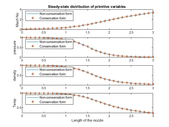
Fig.6: Steady-state distribution of primitive variables inside the nozzle
The variation of `M, p, rho` and `T` at the nozzle is shown in Fig.7. The largest changes take place initially, after which the final, steady-state value is approached.
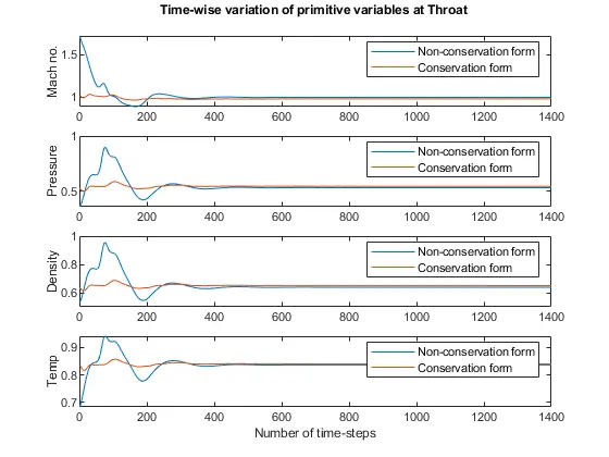
Fig.7: Time-wise variation of the primitive variables at the nozzle throat (i=16 where A=1)
Fig.8 and Fig.9 provide insight into the mechanics of the timewise variation of the flow and its approach to the steady state. The mass flow `rhoVA` is plotted as a function of the distance through the nozzle. 5 different curves are shown, each for a different time during the course of the time-marching procedure. For 50 and 100 time-steps, the mass flow variation simply flops around inside the nozzle due to transient variation of the flow-field variables. However, after 200 time steps, the mass flow distribution begins to settle down, and after 700 time steps, the mass flow distribution is a straight, horizontal line across the graph. This shows that the mass flow has converged to a constant, steady-state value throughout the nozzle. This also satisfies the basic mass flow equation
`rhoVA = constant`
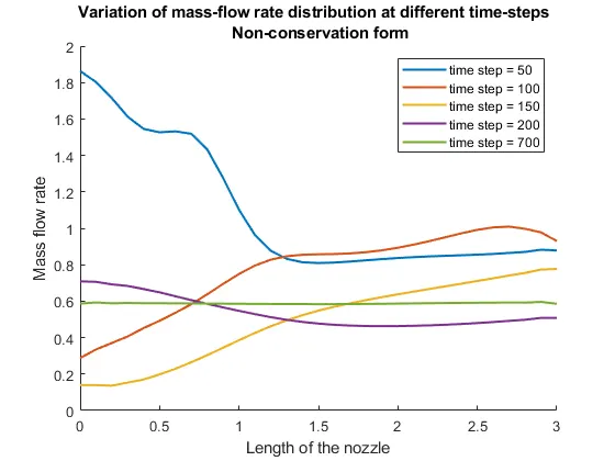
Fig.8: Mass flow rate distribution at different time steps (Non-conservation form)
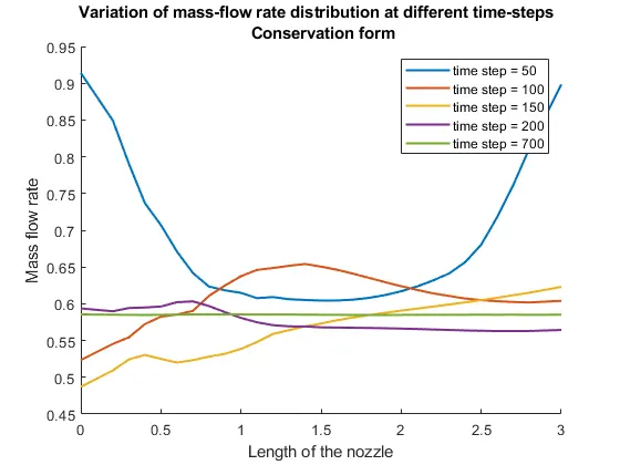
Fig.9: Mass flow rate distribution at different time steps (Conservation form)
Fig.10 demonstrates a general advantage of the conservation form of the equations. The conservation form does a better job of preserving mass throughout the flow field, as the mass flow itself is one of the dependent variables of the equations. On the other hand, the dependent variables in the non-conservation form of the equations are the primitive variables, and the mass flow is obtained only as a secondary result.
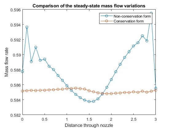
Fig.10: Comparison of mass flow rate distributions for non-conservation and conservation form
Grid Independence:
To check grid independence, the number of grid points is doubled to 61. The figures below show the comparison of the steady-state results for the primitive variables as well as the Mach number at the throat. For the non-conservation form, doubling the number of grid points did improve the numerical solution, but only marginally. The conservation form results come slightly closer to the exact, analytical values, but not as close as the non-conservation form results with half as many grid points. Therefore the non-conservation from results using 31 grid points are essentially grid-independent.
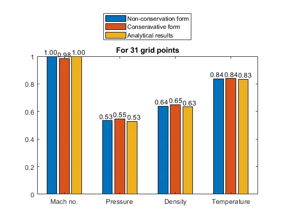
Fig.11: Comparison of the steady state results at 31 grid points
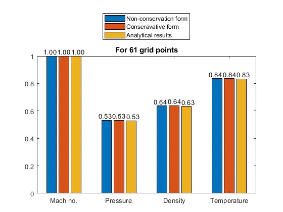
Fig. 12: Comparison of the steady state results at 61 grid points
The behavior of the residuals for the non-conservation form is better than the conservation form.
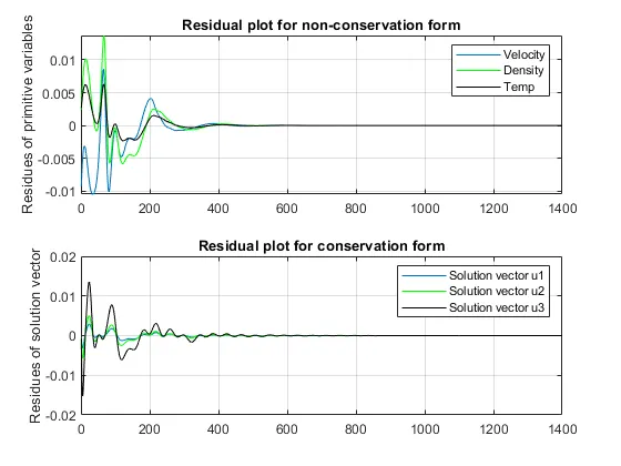
Fig. 13: Behavior of the residuals for non-conservation and conservation form
CONCLUSION:
- The conservation form conserves mass better and thus, this form yields better mass flow distribution.
- The 'Quality' index of numerical algorithms is the amount by which the residuals decay. In this regard, the non-conservation form leads to smaller residuals.
- The non-conservation form produces more accurate results for the primitive variables, whereas the conservation form does this for the flux variables. Thus, there is no clear superiority of one form over the other.