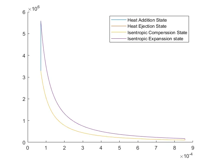
%%
%%%% Writing a program that solve an otto cycle and make plots of it %%%%
%%%%%%%%%%%%%% Using the created function "engine_kinematics"%%%%%%%%%%%%%
clear al
close all
clc
% The theory behaind the calculations is using ideal gas laws
% P1*V1^gama=P2*V2^gama; P1*V1/T1=P2*V2/T2
% Calculating for each states: 1 to 2 (isntropic compression), 2 to 3 (heat
% addition) constant volume, 3 to 4 (isentropic expanssion), 4 to 1 ( heat
% ejection) constant volume

% Inputs, and engine geometry to calculate the volume
P1=101325;
T1=500;
T3=2300;
gama=1.4;
% Engine geometry( bore, stroke, connecting rod, comperssion ratio)
bore=0.1; stroke=0.1; con_rod=0.15;Cr=12;

% Calcualtions for state 1:
% Since we have P1, T1 we need to calculate V1 using engine geometry
% Swep_Volume= PI/4*bore^2*stroke, Clearnace Volume= Swept_Volume/Cr-1
swep_v=(pi/4)*bore^2*stroke;
clearnace_v=swep_v/(Cr-1);
V1=swep_v+clearnace_v;
% Calcualtions for state 2:

% Knowing that V2= clearnce_v, and using P1*V1^gama = P2*V2^gama
% to obtain P2=P1*V1^gama/V2^gama,
% and P1*V1/T1 = P2*V2/T2 to obtain T2=(P2*V2*T1)/(P1*V1);
V2=clearnace_v;
P2=P1*V1^gama/V2^gama;
T2=(P2*V2*T1)/(P1*V1);

% To calculate the changes for both P, and V from state 1 to state 2 need
% to create a function to calculate copmerssion volume, and then obtaining
%compression pressuer, and using the the fact that P1*V1^gama= P1*V2^gama
%constant_C=P1*V1^gama, then comp_pressure = constant_C./comp_volume.^gama;
% The function called engine_kinematics created as matlab function

constant_C=P1*V1^gama;
% Calculating comp_pressure.*comp_volume.^gama = constant_C; from the
% function ceated as "engine_kinematics", then obtaining
% comp_pressure = constant_C./comp_volume.^gama; and theta from 180 to 0

comp_volume=engine_kinematics(bore,stroke,con_rod,Cr,180,0);
comp_pressure = constant_C./comp_volume.^gama;

% Calcualtions for state 3:
% Starting by knowing V3=V2, then calculating P3=(P2*V2*T3)/(T2*V3) from
% ideal gas law, and knowing T3
V3=V2;
P3=(P2*V2*T3)/(T2*V3);

% To calculate the changes for both P, and V from state 3 to state 4 need
% Using the function to calculate expanssion volume, and then obtaining
%expanssion pressuer, and using the the fact that P2*V2^gama= P3*V3^gama
%constant_C=P3*V3^gama, then comp_pressure = constant_C./comp_volume.^gama;
% The function called engine_kinematics created as matlab function

constant_C=P3*V3^gama;
% Calculating comp_pressure.*comp_volume.^gama = constant_C; from the
% function ceated as "engine_kinematics", then obtaining
% comp_pressure = constant_C./comp_volume.^gama; and theta from 0 to 180

expan_volume=engine_kinematics(bore,stroke,con_rod,Cr,0,180);
expan_pressure = constant_C./expan_volume.^gama;


% Calcualtions for state 4:
% Starting by knowing V4=V1, then calculating P4=P3*V3^gama/V4^gama from
% ideal gas law, and claculating T4=(P4*V4*T3)/(P3*V3)
V4=V1;

P4=P3*V3^gama/V4^gama;
T4=(P4*V4*T3)/(P3*V3);

% Polting all states in one plot
hold on
plot([V2 V3],[P2 P3])
plot([V1 V4],[P4 P1])
plot(comp_volume,comp_pressure)
plot(expan_volume,expan_pressure)
% Adding legends to the plot
legend('Heat Addition State', 'Heat Ejection State', ...
 'Isentropic Comperssion State','Isentropic Expanssion state ')