Week 9 - Senstivity Analysis Assignment

INTRODUCTION

The sensitivity analysis in a numerical model is a method in which the effect of change in one or more of the input on the output is analysed. In other words, the expected values of various parameters involved can be used to evaluate the robustness, i.e., ‘sensitivity’ of the results from these changes and identify the values beyond which the results change significantly. In this study, the sensitivity of the temperature on the combustion of methane is analysed using the GRI-3.0 Mechanism.

AIM

Write a code that takes all the reactions from the GRI mechanism and calculates 10 most sensitive reactions. The sensitivity parameter should be with respect to the Temperature.

THEORY

For any reaction to occur there are many intermediate reactions which occurs. In the formation of any products there will be a large number of intermediate steps, some reactions will be slow and some will be very fast. Each of the intermediate steps in the reaction will have different sensitivities to different parameters. Some of the reactions will be sensitive to the concentration of some species, some to temperature, pressure etc. It is important to understand the sensitivity of the reaction to different parameters to control the reaction. A higher sensitivity implies that a small change in one parameter can create a large change in the reaction step.

PYTHON CODE

The python code for sensitivity analysis of the combustion of methane in air is given below:

#%%\
import numpy as np
import cantera as ct 
import matplotlib.pyplot as plt 
#%%
#Initial condition for the reactionmechanism

gas=ct.Solution('gri30.xml')
To=1500
Po=ct.one_atm
gas.TPX=To,Po,{'CH4':0.095,'O2':0.19,'N2':0.714}

#%%
#The reactor network

r=ct.IdealGasConstPressureReactor(gas)
sim=ct.ReactorNet([r])

reaction=gas.reaction_equations()
#print(reac)
N=gas.n_reactions
n=10
S_max=[0]*N
label=[]

for i in range(N):
	r.add_sensitivity_reaction(i)


# set the tolerances for the solution and for the sensitivity coefficients
sim.rtol=1e-6
sim.atol=1e-16

sim.rtol_sensitivity=1e-6
sim.atol_sensitivity=1e-6
states=ct.SolutionArray(gas,extra='t')
reac_num=np.arange(1,N+1)
for t in np.arange(0,2e-3,5e-6):
	sim.advance(t)
	states.append(r.thermo.state,t=t*1000)


	for j in range(N):
		s=sim.sensitivity('temperature',j)
		#plt.plot(t,s)
		if np.abs(s)>np.abs(S_max[j]):
			S_max[j]=s


#%%
#Sorting the arrays

S_abs=np.abs(S_max)
reaction=[a for b, a in sorted(zip(S_abs,reaction),reverse=True)]
reac_num=[a for b,a in sorted(zip(S_abs,reac_num),reverse=True)]
S_max=[a for b, a in sorted(zip(S_abs,S_max),reverse=True)]

#%%
#Extracting the top n sensitive reactions
max_r=reaction[0:n]
max_n=reac_num[0:n]
max_s=S_max[0:n]

#%%
#Extracting mole fractions of species
H_conc=states('H').X
OH_conc=states('OH').X
CH4_conc=states('CH4').X



#plotting
plt.figure(1,figsize=(12,8))
ax1 = plt.subplot()
plt.barh(max_r,max_s,0.4,color='brown')
plt.xlabel('Temperature Sensitivity')
plt.grid( linestyle=':', color='black')
ax1.invert_yaxis()
plt.title(r'Highest Temperature Sensitive Reactions in GRI-3.0 for Stoichiometric Combustion of $CH_4$')
plt.savefig("figsens1.png")


plt.figure(2,figsize=(10,8))
plt.subplot(2,2,1)

plt.plot(states.t,H_conc)
plt.xlabel('Time (ms)')
plt.ylabel(r'$\chi_H$ ')
plt.grid(True)
plt.subplot(2,2,2)
plt.plot(states.t,states.T)
plt.xlabel('Time (ms)')
plt.ylabel('Temperature (K)')
plt.grid(True)
plt.subplot(2,2,3)
plt.plot(states.t,OH_conc)
plt.xlabel('Time (ms)')
plt.ylabel(r'$\chi_{OH}$ ')
plt.grid(True)
plt.subplot(2,2,4)
plt.plot(states.t,CH4_conc)
plt.xlabel('Time (ms)')
plt.ylabel(r'$\chi_{CH_4} $ ')
plt.grid(True)
plt.tight_layout()
plt.savefig("figsens2.png")


plt.show()

The step wise explanation of the above code is given below:

import numpy as np
import cantera as ct 
import matplotlib.pyplot as plt 

The required libraries are imported in this step,

gas=ct.Solution('gri30.xml')
To=1500
Po=ct.one_atm
gas.TPX=To,Po,{'CH4':0.095,'O2':0.19,'N2':0.714}

An instance of the solutions class is made and named gas. The initial temperature is set as 1500K and the pressure as 1 atm. The reactants are initialised as methane and air.

r=ct.IdealGasConstPressureReactor(gas)
sim=ct.ReactorNet([r])

In this snippet a reactor is created and a reactor network is created.

reaction=gas.reaction_equations()
N=gas.n_reactions
n=10
S_max=[0]*N
label=[]

for i in range(N):
	r.add_sensitivity_reaction(i)

In this snippet of code the reactions are taken in an array using the reaction_equation() in the Solutions class. N is the total number of reactions in the mechanism and n is the number of sensitive reactioms we need to extract.

# set the tolerances for the solution and for the sensitivity coefficients
sim.rtol=1e-6
sim.atol=1e-16

sim.rtol_sensitivity=1e-6
sim.atol_sensitivity=1e-6

The simulation tolerances and sensitivity coefficients are set.

states=ct.SolutionArray(gas,extra='t')
reac_num=np.arange(1,N+1)
for t in np.arange(0,2e-3,5e-6):
	sim.advance(t)
	states.append(r.thermo.state,t=t*1000)


	for j in range(N):
		s=sim.sensitivity('temperature',j)
		#plt.plot(t,s)
		if np.abs(s)>np.abs(S_max[j]):
			S_max[j]=s

In this code the reactor networkis advanced each time step and the maximum sensitivity values are stored in an array.

S_abs=np.abs(S_max)
reaction=[a for b, a in sorted(zip(S_abs,reaction),reverse=True)]
reac_num=[a for b,a in sorted(zip(S_abs,reac_num),reverse=True)]
S_max=[a for b, a in sorted(zip(S_abs,S_max),reverse=True)]

The reactions, reaction number and sensitivities are arranged according to the absolute value of sensitivity.

max_r=reaction[0:n]
max_n=reac_num[0:n]
max_s=S_max[0:n]

#%%
#Extracting mole fractions of species
H_conc=states('H').X
OH_conc=states('OH').X
CH4_conc=states('CH4').X

The most sensitive n reactions are extracted and the state of the gas at different time steps are extracted.

#plotting
plt.figure(1,figsize=(12,8))
ax1 = plt.subplot()
plt.barh(max_r,max_s,0.4,color='brown')
plt.xlabel('Temperature Sensitivity')
plt.grid( linestyle=':', color='black')
ax1.invert_yaxis()
plt.title(r'Highest Temperature Sensitive Reactions in GRI-3.0 for Stoichiometric Combustion of $CH_4$')
plt.savefig("figsens1.png")


plt.figure(2,figsize=(10,8))
plt.subplot(2,2,1)

plt.plot(states.t,H_conc)
plt.xlabel('Time (ms)')
plt.ylabel(r'$\chi_H$ ')
plt.grid(True)
plt.subplot(2,2,2)
plt.plot(states.t,states.T)
plt.xlabel('Time (ms)')
plt.ylabel('Temperature (K)')
plt.grid(True)
plt.subplot(2,2,3)
plt.plot(states.t,OH_conc)
plt.xlabel('Time (ms)')
plt.ylabel(r'$\chi_{OH}$ ')
plt.grid(True)
plt.subplot(2,2,4)
plt.plot(states.t,CH4_conc)
plt.xlabel('Time (ms)')
plt.ylabel(r'$\chi_{CH_4} $ ')
plt.grid(True)
plt.tight_layout()
plt.savefig("figsens2.png")


plt.show()

The figures are plotted using the above code.

RESULTS AND DISCUSSION

The results of the above simulation is given below:

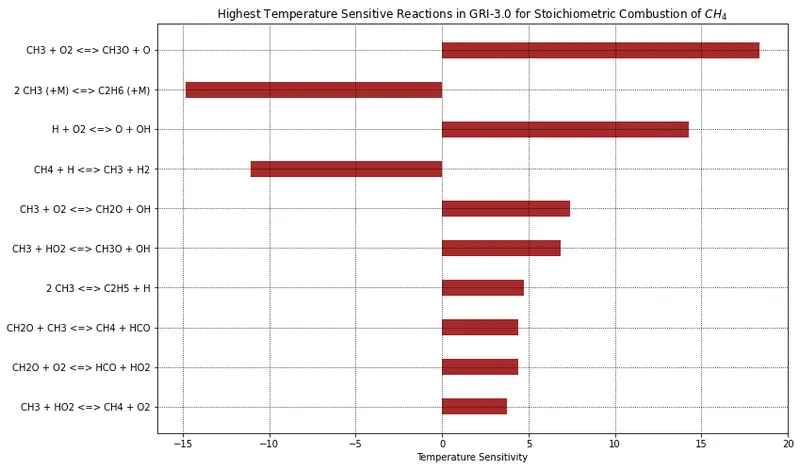
These are the top 10 reactions which are more sensitive to the change of temperature. It can be seen that the sensitivity has both positive and negative values. The positive sensitivity implies that if the temperature is increased the reaction rate increases for that particular reaction. For negative sensitivity if the temperature increases the reaction rate decreases.

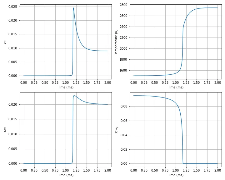
In this figure at first the initial concentration of the species `H` and `OH` is zero and `CH_4` is as the initial condition given. The change in the concentrations and temperature is very rapid but takes place after some time which represents the ignition delay.

From the above figure it can be seen that the temperature stabilises at a higher value, the mole fraction of the species also stabilises which implies that the reaction reached an equilibrium. The `CH_4` is completly consumed but there are `H` and `OH` species present even after the fuel is burned completly.

CONCLUSION

The sensitivity analysis shows that reactions shows positive and negative sensitivities to temperature. A positive sensitivity implies that an increase in temperature will increse the rate of that reaction. When the sensitivity is negative, an increase in temperature will reduce the rate of the reaction.

The second plots represents the ignition delay of the combustion reaction. The sharp dip or rise represent the ignition process which is very instantaneous in naure.