Week 9 - Senstivity Analysis Assignment

OBJECTIVES :- To analyse sensitivity with respect to the temperature.

PROBLEM STATEMENTS :-

Write a code that takes all the reactions from the gri mechanism and calculate 10 most sensitive reactions.

The sensitivity parameters should be with respect to the temperature.

Our program should show the reaction strings in the order of greatest sensitivity to the least sensitivity.

Our program should be parametric, it is should be intutive and easy to obtain "n" number of sensitive reaction with respect to the asked parameters, by simply changing a number.

For additional points plot a graph of sensitivities vs the reaction.

THEORY AND INTRODUCTIONS :-

Sensitivity analysis for Nonlinear heat conductions :-

Parameters in the heat conduction equation are frequently modeled as temperature dependent. Thermal conductivity, volumetric heat capacity, convection coefficient, emmisivity and volumetric source terms are parameters that may depends on temperature. Many applications, such as parameter estimations, optical experimental design, optimization and uncertainity analysis, require sensitivity to the parameters describing temperature dependent proparties. A general procedure to compute the sensitivity of the temperature field to model parameters for nonlinear heat conduction is studied. Parameters are modeled as arbitrary function of temperature. Sensitivity equations are implimented is an unstructured grid, element based numerical solver. The objectives of this study are to describe the methodology to derive sensitivity equation for the temperature-dependent parameters and present demonstrations calculations. In addition to a verification problem, the design of an experiment to estimate temperature variable thermal proparties is discussed.

IMPORTANCE OF SENSITIVITY ANALYSIS :-

Sensitivity analysis is a method for predicting the outcome of a decision if a situation turns out tobe different compared to the key predictions. It helps in assessing the riskiness of a strategy. Helps in identifying how dependent the output is on a particular input value.

The various techniques widely applied include-

• Differential sensitivity analysis
• One at a time sensitivity measures
• Factorial analysis
• Correlation analysis
• Regression analysis
• Subjective sensitivity analysis

Using Sensitivity Analysis for decision making :-

One of the key applications of sensitivity analysis is in the utilizations of models by manegers and decision makers. All the content needed for the decision model can be fully utilized only through the repeated applications of sensitivity analysis. It helps decision analysts to understand the uncertainities, pros and cons with the limitations and scope of a decision model.

Most if not all decision are made under uncertainity. It is the optimal solution in decision making for various parameters that are approximations. One approach to come to conclusion is by replacing all the uncertain parameters with expected values and then carry out sensitivity analysis. It would be a breather for a decision maker if he has some indication as to how sensitive will the choices be with changes in one or more inputs.

Uses of Sensitivity analysis :-

• The key application of sensitivity analysis is to indicate the sensitivity of simulation to uncertainities in the input values of the model.
• The help in decision making
• Sensitivity analysis is a method for predicting the outcome of a decision if a situation turns out tobe different compared to the key predictions.
• It helps in assessing the riskiness of a strategy
• Helps in identifying how dependent the output is on a particular input value. Analysis of the dependency in turn helps in assessing the risks associated
• Helps in taking informed and appropriate decisions
• Aids searching for errors in the model.

STEP WISE EXPLAINATION OF THE CODE :-

1. First off all I imported the required module to take required data from their library.
2. then specify the gas as a solutions of "gri30" mechanism.
3. then define the temperature & pressure value
4. then define the mole fraction are CH4, O2 & N2
5. then use the suitable reactor as "Ideal Gas Constant Pressure Reactor" and specify the gas n it.
6. then specify the reactor network for simulations.
7. then specify the reactions for reaction equation.
8. then specify more sensitive to the temperature reactions, here i.e. N=10
9. then specify total number of gas reactions here i.e."n"
10. we can change here "n" by any number to showing the that number of reactions.
11. use the linspace command to specify the range and type is intiger
12. use the for loop to specify the reactions range.
13. then set the relative and absolute tollerance for rector network & sensitivity.
14. sensitivity tollerance always greater than reactor netwok tollerance.
15. then specify the temperature as "T" and arrange it from 0 to 2ms, by taking interval as 0.005 ms
16. define states in the form of solution array
17. for sorting the reaction from higher rate to lower rate use "zip" command
18. sorting the reactions, reactor id & sensitivity.
19. specify the empty array for new sensitivity & new names and append it higher reactive sensitivity & names
20. use the spacing in new names & new sensitivity i %s & %f
21. ordinate i.e obscissa sorted in "min value -1, max value + 1, length" and reverse it, i.e. (N, 0, -1)
22. then plot the horizontal bar graph of ordinate, new sensitivity & new names.
23. use figure size = (20,5) & font size = 6
24. then plot another figure by taking subplots are temperature vs time, OH mole fraction vs time, H mole fraction vs time, CH4 mole fraction vs time.
25. and finaly show it.

SENSITIVITY CODES :-

import sys
import numpy as np 
import cantera as ct 
import matplotlib.pyplot as plt 

gas = ct.Solution("gri30.xml")
temp = 1500
press = ct.one_atm
gas.TPX = temp, press, {"CH4":1, "O2":2, "N2":7.52}
r = ct.IdealGasConstPressureReactor(gas, name = "R1")
sim = ct.ReactorNet([r])
reactions = gas.reaction_equations()

# List of reactions
N = 10
n= gas.n_reactions
rid = np.linspace(1,n,n).astype(int)

# Enable sensitivity with respect to the rates of the n
# Reactions (Reactions 0 through n)
for i in range(n):
	r.add_sensitivity_reaction(i)

# Set the tollerances for the solution and for the sensitivity coefficients
sim.rtol = 1e-6		# relative change in solution should be less than this number
sim.atol = 1e-15 	# absolute change in solution should be less than this number

sim.rtol_sensitivity = 1e-6		# relative change in sensitivity should be less than this number
sim.atol_sensitivity = 1e-6		# absolute change in sensitivity should be less than this number

sensitivity = np.zeros(n)
names = []

T = np.arange(0, 2e-3, 5e-6)
states = ct.SolutionArray(gas, extra = ["time_in_ms", "t"])
	
for j in T:
	sim.advance(j)

	for k in range(n):
		states.append(r.thermo.state, time_in_ms = 1000*j, t=j)
		s = sim.sensitivity("temperature", k)
		names.append(sim.sensitivity_parameter_name(k))
		if np.abs(s) >= np.abs(sensitivity[k]):
			# Storing maximum values
			sensitivity[k] = s 	

# Sorting the reactions & reaction ID's based on absolute value of sensitivities
reactions = [r for s, r in sorted(zip(np.abs(sensitivity), reactions), reverse=True)]
rid = [r for s, r in sorted(zip(np.abs(sensitivity), rid), reverse=True)]
sensitivity = [s for abs_s, s in sorted(zip(np.abs(sensitivity),sensitivity), reverse=True)]

# Extracting the top 10 sensitive reactions
new_sensitivity = []
new_names = []

for l in range(N):
	new_sensitivity.append(sensitivity[l])
	new_names.append(names[l])

for m in range(N):
	print("%s = %f" %(new_names[m], new_sensitivity[m]))

# Obscissa = sorted(list(np.linspace(min_value-1, max_value+1, length)), reverse = True)
ordinate = list(np.arange(N,0,-1))

plt.figure(1)
plt.figure(figsize = (20, 5))
plt.barh(y = ordinate, width = new_sensitivity, tick_label = new_names, color = ["black","brown"], height = 0.5)
plt.yticks(fontsize = 6)
plt.ylabel("sensitivity value")
plt.title("Top ten sensitivity values for temperature")

# Plots the results if matplotlib is installed
# see http://matplotlib.org/ to get it
plt.figure(2)
plt.subplot(2,2,1)
plt.plot(states.t, states.T)
plt.xlabel("Time(ms)")
plt.ylabel("Temperature (K)")
plt.subplot(2,2,2)
plt.plot(states.t, states("OH").X)
plt.xlabel("Time(ms)")
plt.ylabel("OH mole fraction")
plt.subplot(2,2,3)
plt.plot(states.t, states("H").X)
plt.xlabel("Time (ms)")
plt.ylabel("H mole fraction")
plt.subplot(2,2,4)
plt.plot(states.t, states("CH4").X)
plt.xlabel("Time (ms)")
plt.ylabel("CH4 mole fraction")
plt.tight_layout()

plt.show()

RESULTS :-

From above code we get following results are-

1. Top 10 sensitivity value for temperature :-

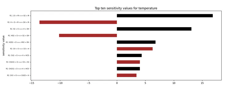
abobe horizontal bar graph showing highest sensitive reactions. Right side bar showing positive temperature reactions and left side bar showing negative temperature reactions. Positive temperature are faster rates than negative temperature. This bar graph is very helpful to showing which rection rate is very faster and which reaction rate is slower. Here showing higher and lower rates, which are very sensitive in all sensitivity reactions.

2. Subplots :-

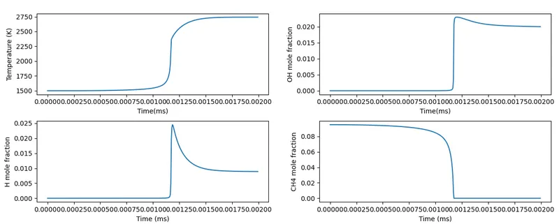
Here have four different graphs are-

1. Temperature Vs time :- Picture showing 1 ms delay time for combustion at 1500k, thereafter it increases tremendously and kept constant at higher value of temperature.
2. OH mole fraction vs time :- Here have same delay period and then increases mole fraction aand then goes down slowlly.
3. H mole fraction vs time :- The result is similar to "OH mole fraction vs time" but, at last decreasing at higher rate.
4. CH4 mole fraction vs time :- First off all mole fraction is higher upto certain time, then it decreases and finally it kept constant at zero upto end time.

3. Top 10 sensitive reactions :-

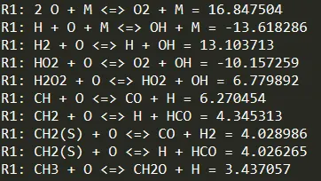
Above output showing 10 different faster rate sensitive reactions in negative or positive rates. Negative value showing slower reaction rate and positive value showing higher reaction rate. The value of higher reaction rate i.e. "2*O + M -> O2 + M" = 16.847504 and the value for lower reaction rate i.e. "H + O + M -> OH + M" = -13.618286. Other reaction are in mean reaction rate as shown in above output snapshots. Above reactions are output of the code which I written for sensitivity.

CONCLUSIONS :-

From above code and results we can conclude following points are-

1. We can change any number of rates of reactions, only by replacing "n" to any digit in the above code.
2. We can change the reactor according to our solution and mole fraction.
3. For sensitivity we consider two tollerance i.e. relative tollerance & absolute tollerance
4. Here absolute tollerance for sensitivity is greater than absolute tollerance for solutions.
5. For sorting reactions and reaction ID's, we can use "zip" solver here.
6. Here new sensitivity is our higher rates of sensitivity of reactions.
7. here, ordinate showing the arrangement of the list.
8. here, command barh is nothing but the horizontal bar command.
9. barh command is used for to showing sensitivity values for temperature.
10. Subplot is used for showing all mole fraction graph in single graph.
11. Sensitivity values showing it's order of rate in that reactions.
12. In bar graph, Left side bar showing negative values means lower sensitivity while right side bar showing positive values means higher sensitivity.
13. Subplot showing the delay in combustion.
14. Output of the code showing the value of each sensitivity.

In this way, I write the code that takes all reactions from the GRI mechanism & calculate 10 most sensitive reactions. Also write the sensitivity parameter should be with respect to the temperature. zip command is used for reaction strings in the order of greatest sensitivity to the least sensitivity. And finally we get the successful results for concluding.