Parametric study on Gate valve

Aim:-

• Perform a parametric study on the gate valve simulation by setting the opening from 10% to 80%.
• Find out the mass flow rate at the outlet for each design point.
• Calculate the flow coefficient and flow factor for each opening and plot the graph.
• Discuss the result on the mass flow rate and flow coefficient.

Objective:-

• Load and extract the required fluid volume in the space claim.
• Set the parametric definition for the opening of the gate valve in the space claim.
• Mesh the model in the mesh module of the fluent cell.
• Simulate the simulation for a specified percentage on the opening of the gate.
• Obtain the mass flow rate at the outlet of the gate valve for each case.
• Use parametric setting to generate results for other percentages of opening setup.
• Calculate the flow coefficient and flow factor for each opening and plot the graph.
• Discuss the results of the mass flow rate and flow coefficient.
• Write a well-defined report with all the necessary details.

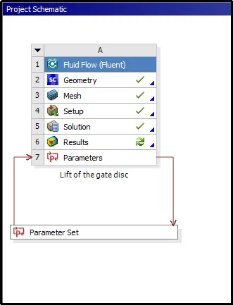
In this project, the parametric simulation of the gate valve is performed by controlling or changing the position of the gate of the valve using the Ansys parametric setting. This simulation is important to study the flow rate of the fluid with different levels of lift of the gate disk.

A gate valve, also known as a sluice valve, is a valve that opens by lifting a barrier (gate) out of the fluid. Gate valves require very little space along the pipe axis and hardly restrict the flow of fluid when the gate is fully opened. The gate faces can be parallel but are most commonly wedge-shaped (to be able to apply pressure on the sealing surface).

Geometry setup:-

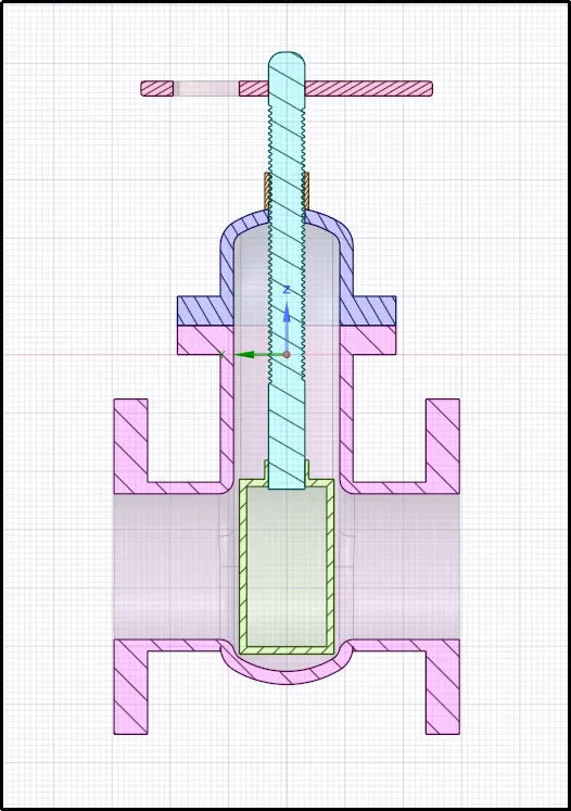
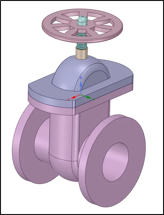
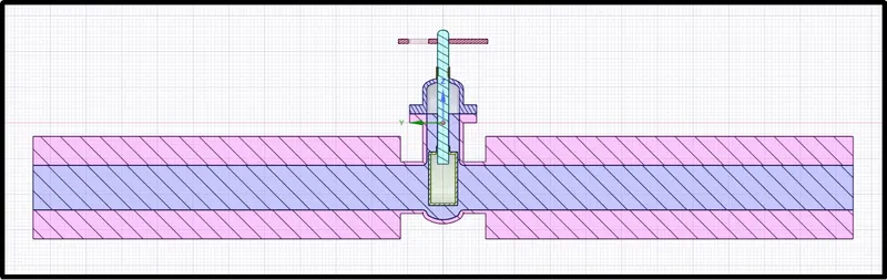
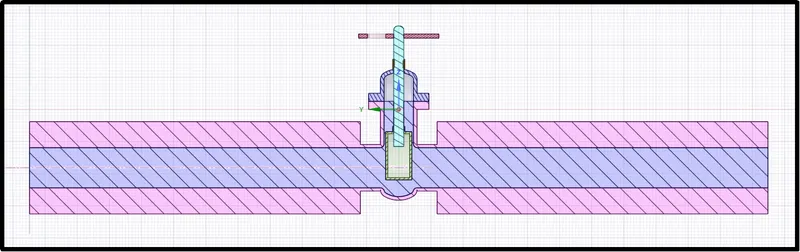
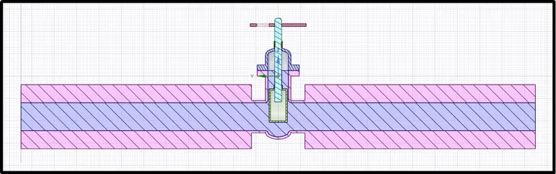
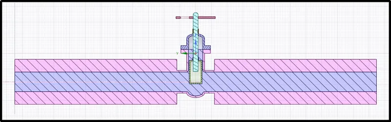
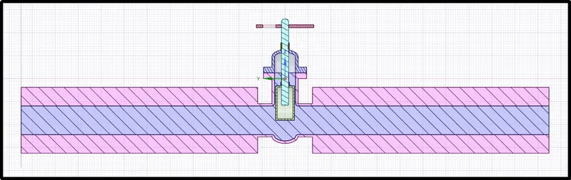
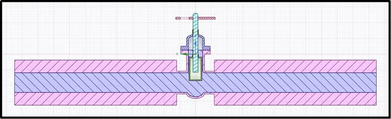
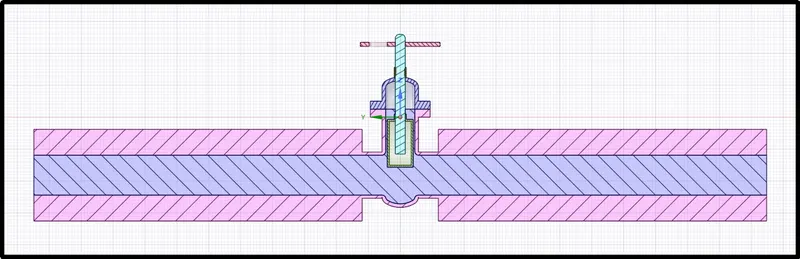
In this simulation, Ansys Space claim was used for geometry setup and the following model was used to perform the analysis. The gate valve consists of a hand wheel and a spindle that is connected to the gate disk inside the casing of the gate valve. The valve has two open ports - one for the inlet and another for the outlet of the fluid.

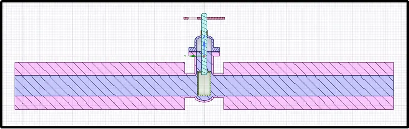
In the Ansys Space claim first, the model was set up by extracting the fluid volume from the component. Inlet and outlet ports were pulled by 800mm to observe the fluid flow properly. Furthermore, the threaded portion of the rod was defeatured to avoid mesh failure and fluctuation in simulation results. Finally, adapt fluid volume to changing solid geometry.

This simulation is performed to understand the parametric study to analyze the flow rate at the outlet of the gate valve through different levels of the lifts of the gate disk. Therefore parameters of the lifts of the gate disk were activated by using the move command, which allowed us to select and move bodies or components. While moving component it asks us to input dimensions, additionally, it also asks us to set this dimension as a parametric value by showing the ‘P’ sign on the right side of the dimension. Using this setting we can set parametric dimensions.

To edit those parametric dimensions, one can just select the group panel and can change ruler dimensions.

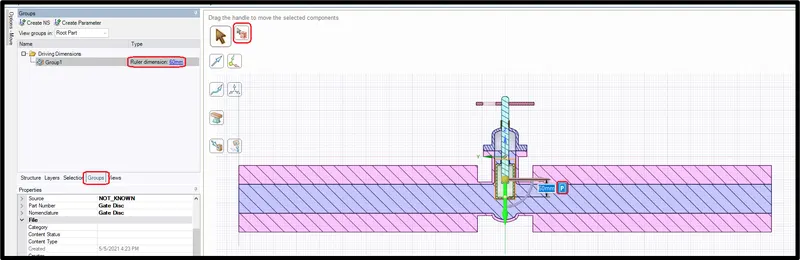
(for this example 10% lift of the gate is considered)

Meshing:-

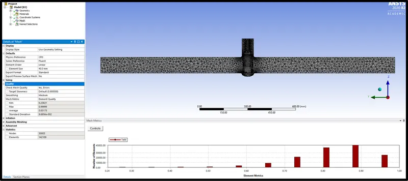
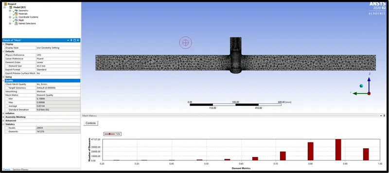
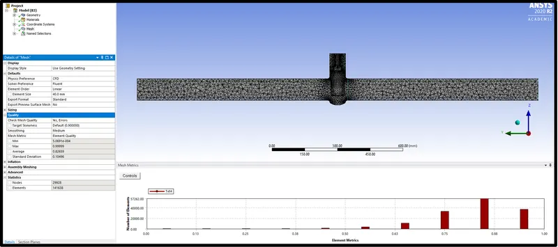
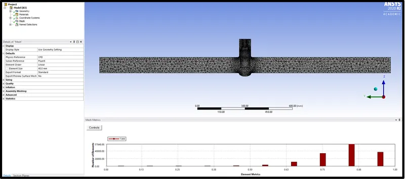
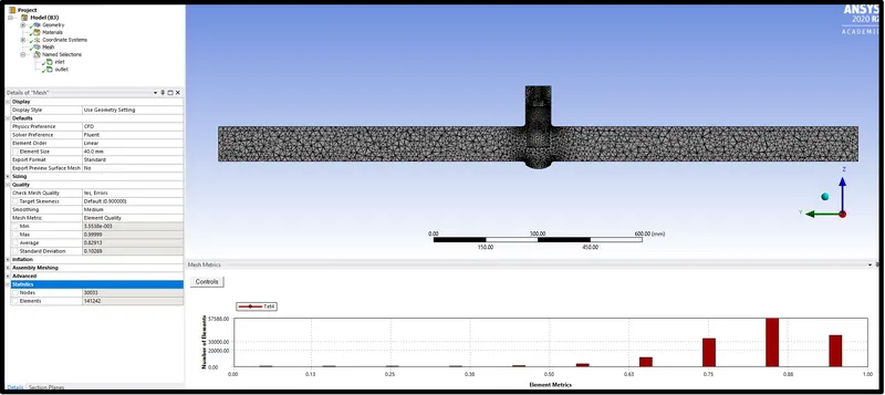
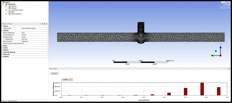
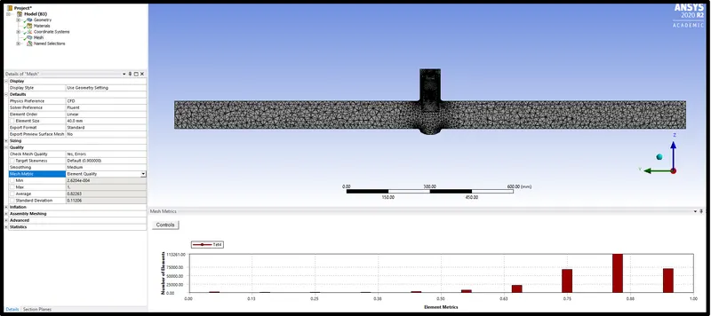
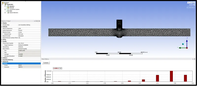
The geometry model was meshed using 40mm of average mesh size and mas mesh size of 80 mm. The curvature and proximity were turned on to implement a fine meshing neat curve and thin area respectively.

Boundary name:-

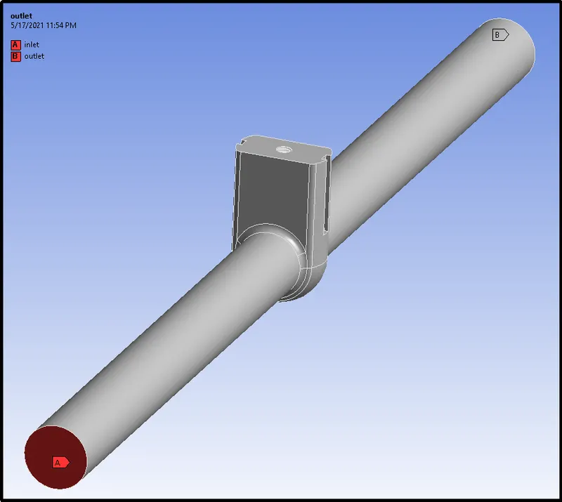
The fluid volume only has two open port inlet and outlet, hence, boundary names were provided as depicted in the following figure.

Fluent Setup:-

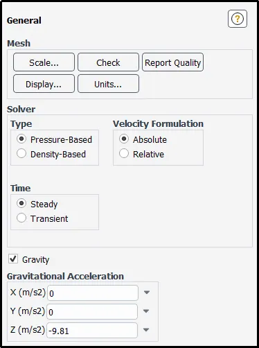
In this study, gravity was turned on in a negative z-direction. A pressure-based solver was used with absolute Velocity formation considering the steady-state condition.

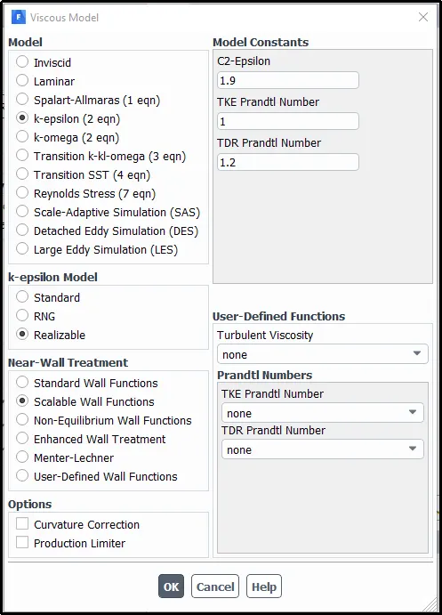
For this type of case, we are going to use a k-epsilon - a realizable model with a scalable wall function.

Scalable wall function:- This function is applicable for the meshes with even Y+ 1. But still, it is a wall function. The only purpose of scalable wall function is to avoid problems of successive refinements in standard wall function meshes. The algorithm ensures that your solver Y+ (Y* in Fluent) is always greater than 11.225. Y+= 11.225 is the intersection of linear and log law profile. It has a function that chooses the maximum of (11.225, Y*).

Material selection:-

Fluid material was selected as water-liquid from a fluent database.

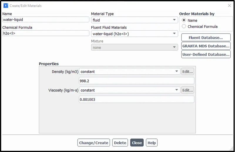
Material definition:-

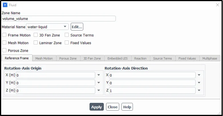
In cell zone condition the working fluid is set to the water liquid.

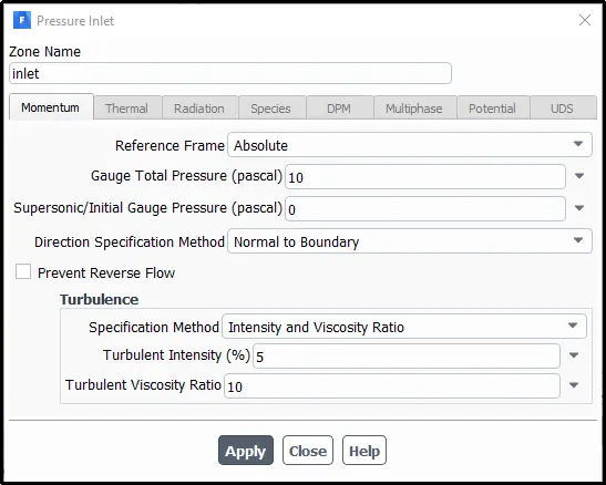
Boundary Condition:-

In this particular case, the pressure base inlet boundary condition was selected. Typically, for pipe flow, 10-pascal pressure is considered, hence, 10-pascal gauge pressure was given at the inlet.

Mass flow rate Definition:-

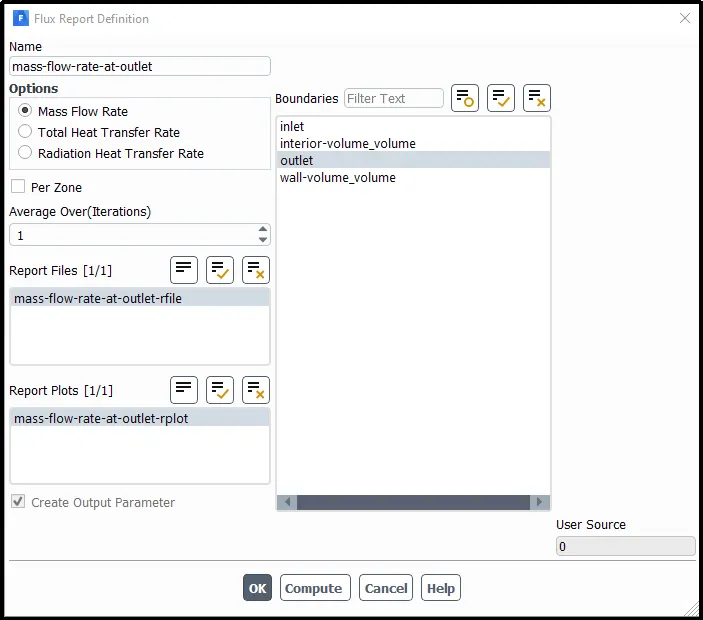
To plot the mass flow rate at the outlet port mass flow rate definition was created in fluent to plot and print the results and the output parameter was also turned on to simulate the model for the various lift of the gate disc.

Solution Initialization:-

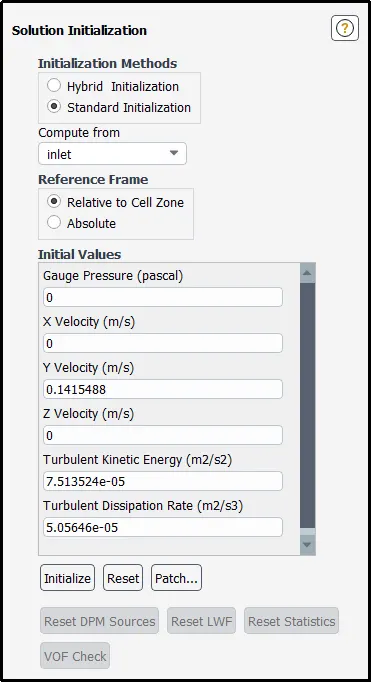
Solution setup was initialized by using standard initialization process as in this problem all surfaces boundary is already defined. The solution was initialized from the inlet.

Solution Convergence:-

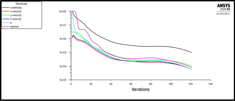
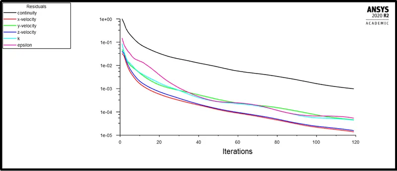
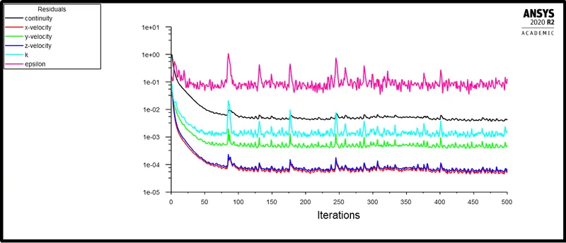
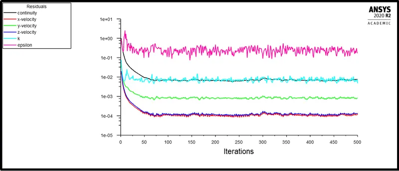
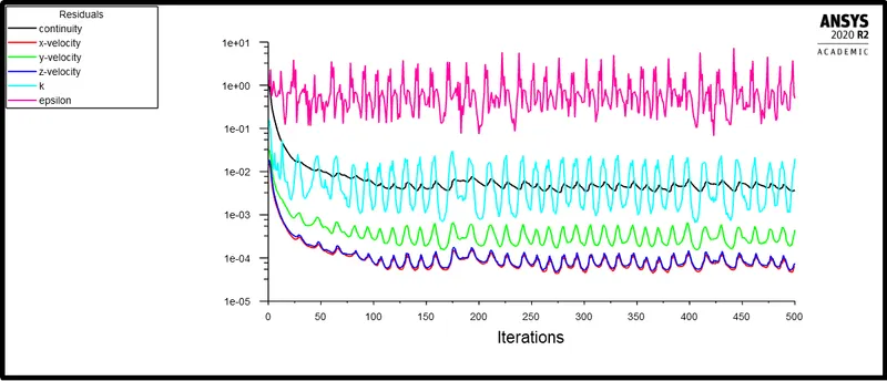
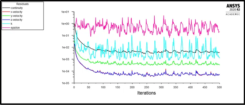
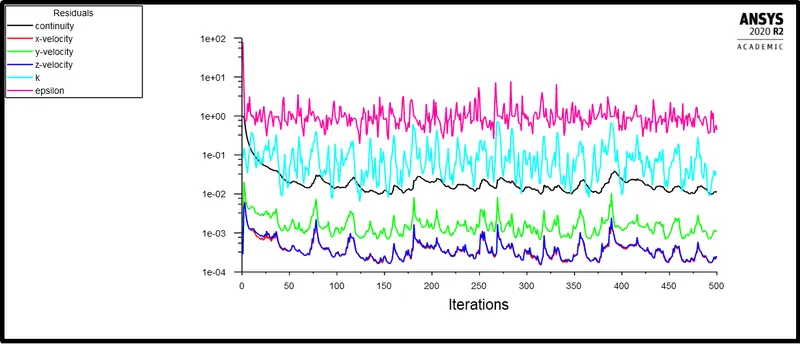
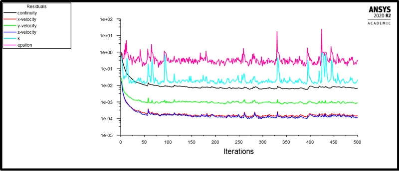
Solution set to run for 500 iterations but it converging at 124^th iteration. The following plot shows the residual plot for the above simulation of 10% lift of the gate disc

Mass flow rate at the outlet of the gate valve:-

Mass flow rate is getting stable after 25 iteration which shows the iterative solutions are converged.

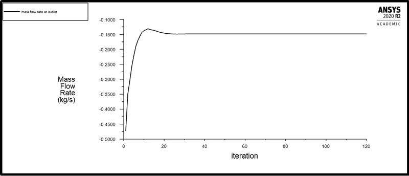
Mass flow rate at outlet for the 10% lift is 0.14850942kg/s

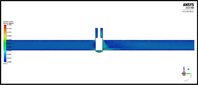
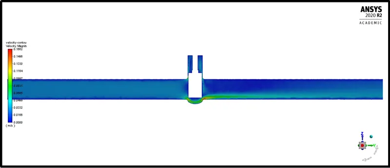
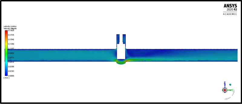
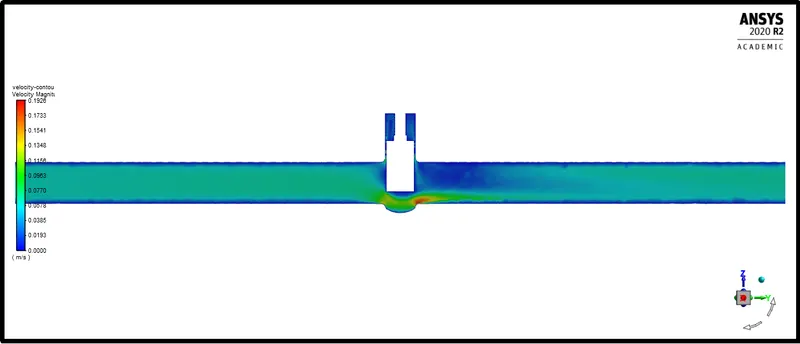
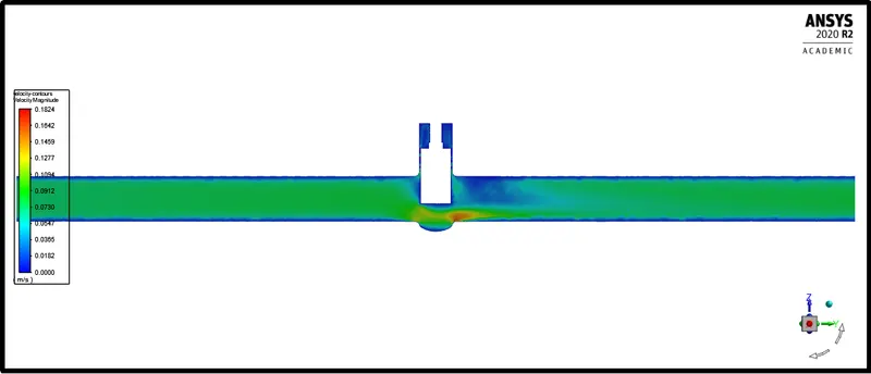
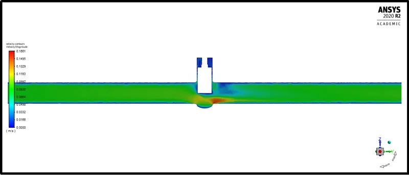
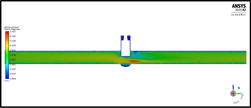
Velocity contour:-

The flow coefficient:-

The flow coefficient of a device is a relative measure of its efficiency at allowing fluid flow. It describes the relationship between the pressure drop across an orifice valve or other assembly and the corresponding flow rate.

Mathematically the flow coefficient C_v (or flow-capacity rating of the valve) can be expressed as:

`C_v = Q sqrt((SG)/(Delta P))`

Where

Q is the rate of flow (expressed in US gallons per minute),

SG is the specific gravity of the fluid (for water = 1),

`Delta P` is the pressure drop across the valve (expressed in psi).

For 10 mm lift of the gate disc

Q = 0.00014772 m³/s = 2.34141 gpm

SG = 1

`Delta P` = inlet pressure - outlet pressure = 10 - 0.18427 = 9.81573 Pa = 0.001423651273 psi

`C_v = 2.34141 sqrt((1)/(0.001423651273))`

`C_v = 62.05483`

Flow factor:-

The metric equivalent of the flow coefficient - `C_v` - is based on the SI-system and is called the flow factor (`K_v`)

The flow factor (K_v) is defined as the flow of water with temperature ranging 5 - 30̊C through a valve in a valve in cube meters per hour(`m^3`/h) with a pressure drop of 1 bar.

The relationship between `C_v` and `K_v` can be expressed as:-

`C_v = 1.16 K_v`

`K_v = 0.862 C_v`

`K_v = 0.862 xx 62.05483`

`K_v = 53.49126`

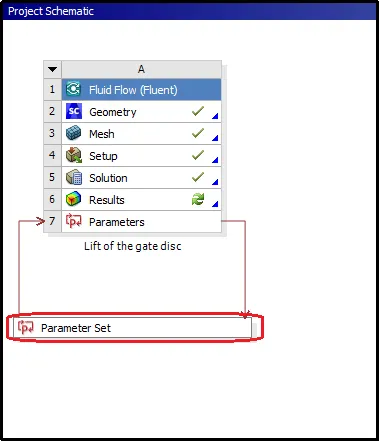
To calculate mass flow rate, flow coefficient, and flow factor for other parametric positions of the gate disk one can simply use parametric setup and click update.

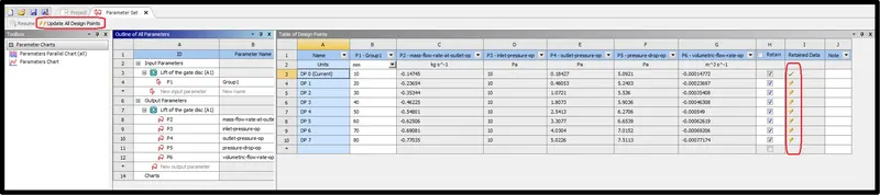
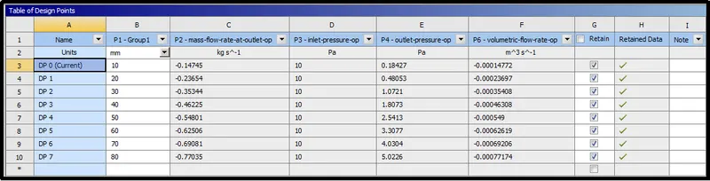
After hitting update all design points it will solve the solution for all lift positions of the disc.

For 10% lift of the gate disc:-

Mass Flow Rate (kg/s)
-------------------------------- -------------------
outlet -0.14744942

For 20% lift of the gate disc:-

Mass Flow Rate (kg/s)
-------------------------------- -------------------
outlet -0.23654463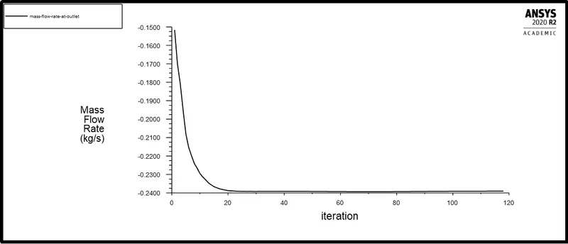

For 30% lift of the gate disc:-

Mass Flow Rate (kg/s)
-------------------------------- -------------------
outlet -0.35344358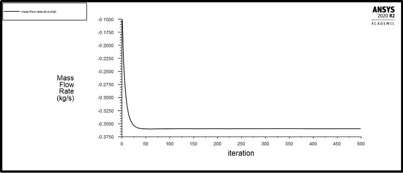

For 40% lift of the gate disc:-

Mass Flow Rate (kg/s)
-------------------------------- -------------------
outlet -0.4622851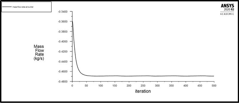

For 50% lift of the gate disc:-

Mass Flow Rate (kg/s)
-------------------------------- -------------------
outlet -0.54801886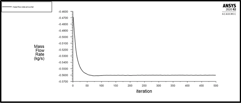

For 60% lift of the gate disc:-

Mass Flow Rate (kg/s)
-------------------------------- -------------------
outlet -0.62506161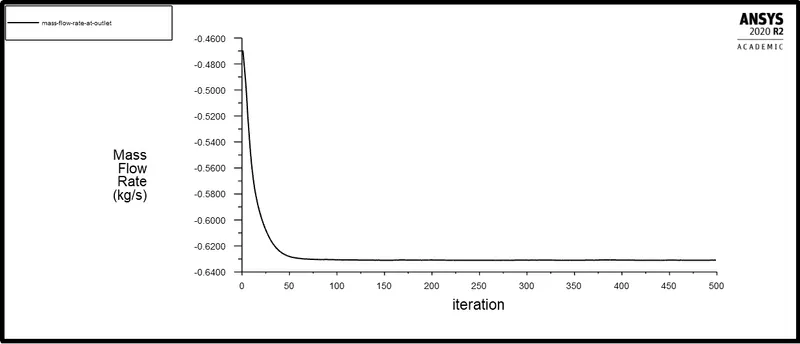

For 70% lift of the gate disc:-

Mass Flow Rate (kg/s)
-------------------------------- -------------------
outlet -0.69018214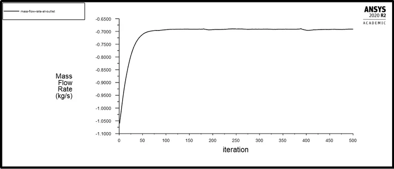

For 80% lift of the gate disc:-

Mass Flow Rate (kg/s)
-------------------------------- -------------------
outlet -0.77035201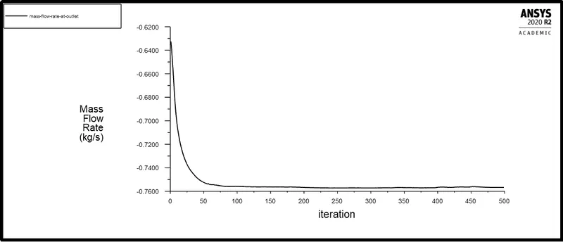

Variation in mass flow rate as the gate opens:-

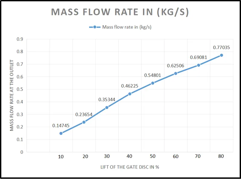
The above chart portrays the variation of mass flow rate with changes of lift of the gate disc. A glimpse over the graph exhibits that the mass flow rate at the outlet of the gate valve increasing as the valve opens up more and more.

Result Table:-

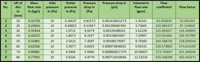
The above observation table exhibits the changes or variation in mass flow rate values at the outlet port as the gate valve disc lift upwards. It then shows the calculated values of the flow coefficient and flows factor.

Variation in flow coefficient and flow factor:-

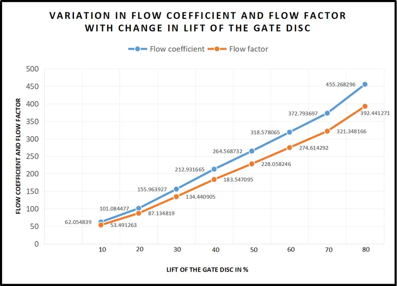
As we saw in the mass flow rate graph before, both, flow coefficient and flow factor values also increases as the mass flow rate at the outlet increases.

Conclusion:-

• Using parametric setup for geometry in the Ansys workbench we can save more time and reduce efforts in simulation for changing geometrical conditions.
• low lift of the gate disc leads to higher pressure drop and as the gate vale opens the pressure dorp reduces.
• Mass flow rate at the outlet increases as the lift of the gate disc rises or the valve opens.
• The flow coefficient and flow factor also increases as the mass flow rate at the outlet port increases.