Week - 9 Material modeling from raw data

Aim: Use the diagram of the true stress-strain curve of graphite iron casting, pick any one of them and use the data to create either a MAT_024 or MAT_018 material model, and then validate it.

Work flow:

1. Extract the data from the plot
2. Clean the data and visually confirm that it matches the original data and the elastic modulus is 20.9E+06 psi.
3. Convert the data to (kg-mm-ms) unit system
4. Process the data and create the material as demonstrated
5. Use the material model with a dogbone specimen and validate the same.

Procedure:

1. In order to extract the data from the plot, data digitizer is used, and the x and y-axis limit is marked and also pointers are marked through the curve selected and the stress-strain data is exported to excel.
2. Now, the stress-strain values that one gets through any material testing plots are generally engineering stress and engineering stress values, Thus this stress-strain curve is plotted and then we can notice that there are many anomaly points or irregular points or noice which may affect once the data is feed into ls dyna. So, curve fitting is done to oclean the data, ytendline is set by using logarithmic scale by using R squared value of 0.9889.
3. Now , as mentioned above ,the stress-strain values that one gets through any material testing plots are generally engineering stress and engineering stress values, and also the stress unit that we got from the curve is ksi which is changed into Mpa , wher3, 1ksi =6.89476 Mpa.
4. Now , we have Engineering stress Vs engineerng strain value, that we plotted as shown below.

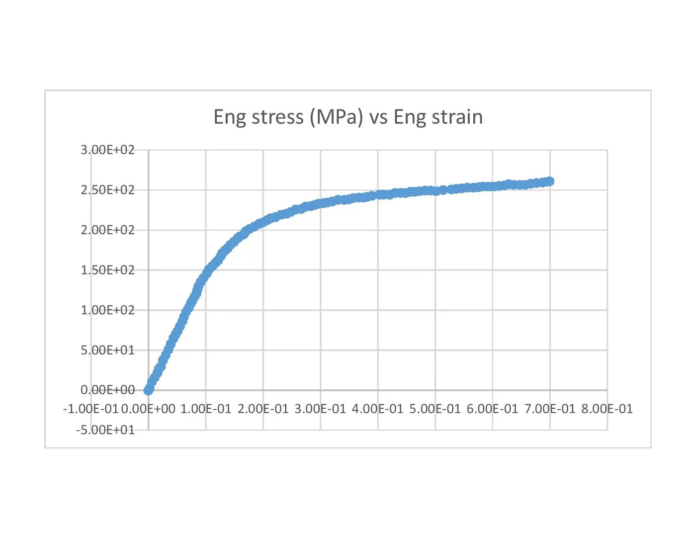5. Now It is converted to True strain and true stress and then effective plastic strain is calculated using below shown formula:

True strain = ln(1 + engineering strain)

True stress = (engineering stress) * exp(true strain) = (engineering stress) * (1 + engineering strain)

effective plastic strain (input value) = total true strain - true stress/E, Wher E is in Gpa, which is found to be 144 Gpa.

The plot of Effective plastic strain Vs effective stress is shown below:

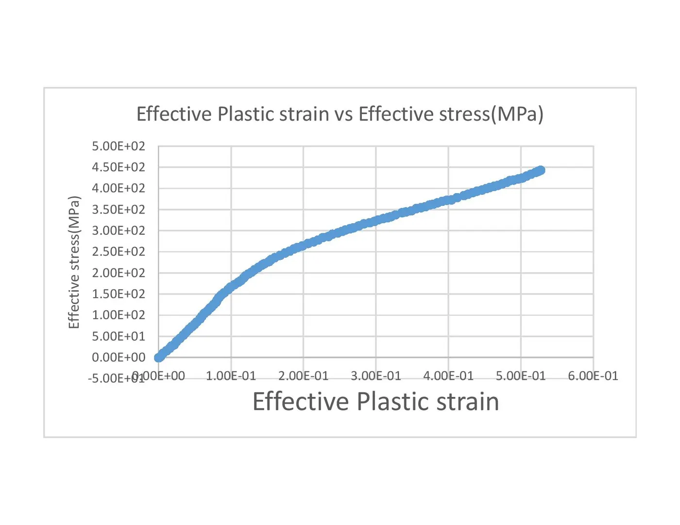6. Now as we now have the Effective plastic strain vs effective stress values, we now use this data to define a curve that we named as material curve which would be used to define our MAT24.

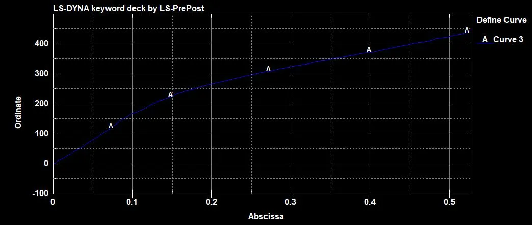Fig : The material curve plot that was given as input

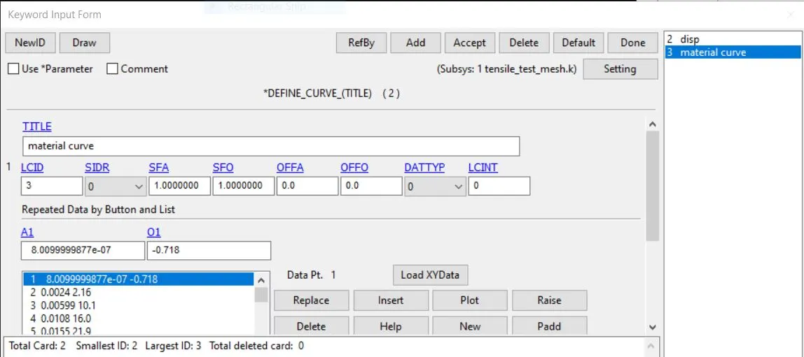
Once the material card has been created, it has to be implemented. SO, first we load the dogbone specimen provided and the define the section shell with ELFORM 16 and thickness of shell 1.5mm and then define the part with the shell section and the material card created.

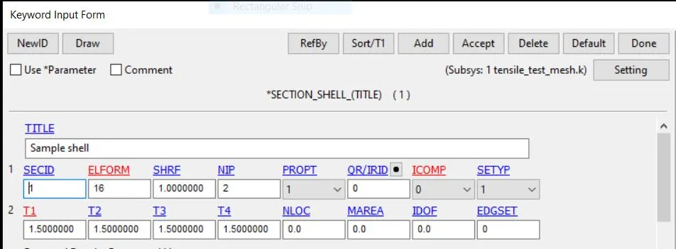
Fig: section shell card

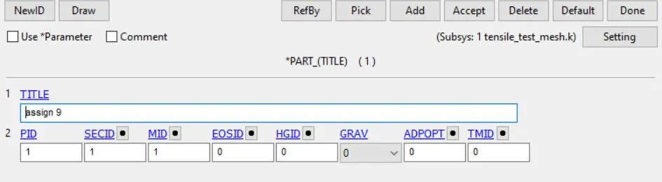Fig : Part card

Now, as we have to do a tensile simulation. Proper boundary condition has to be implemented.

1. We used SPC set, in one edge so that that end is fixed, (to compare with the sample being gripped), and keep it non constrained only in y translational direction (direction perpendular to the displacement provided in th expt)

2. Also the mid node on the two opposide edges are constrained in only the y translational and rotation about all axis.

3. A prescibed boundary motion is applied on the opposite edge of the gripped boundary, and a displacement curve is defined.

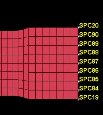
Fig : SPC on one edge

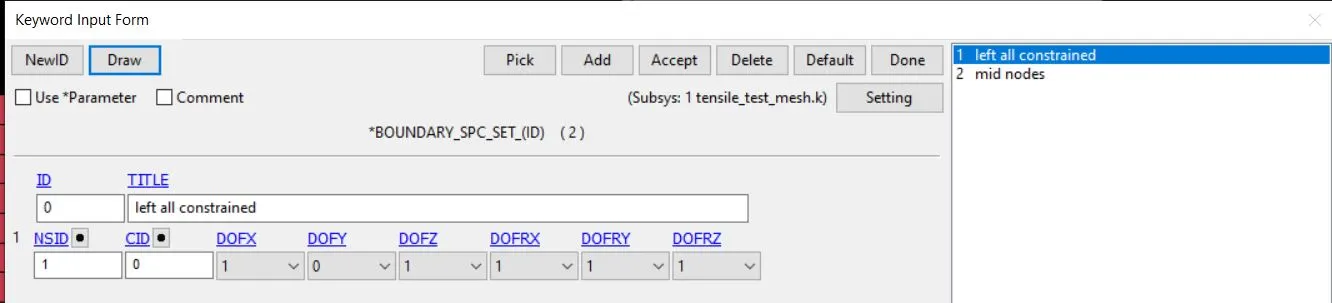
Fig : SPC on one edge card

Fig:boundary spc mid node model

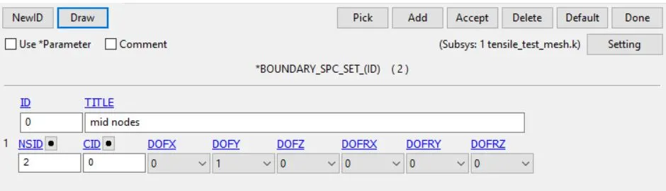
Fig:boundary spc mid node card

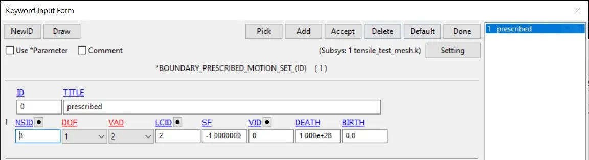Fig:boundary prescribed card.

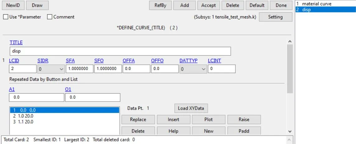FIg: Displace curve that was used in boundary prescribed sets.

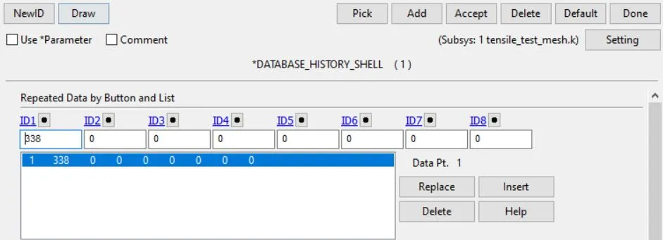Fig: History shell was defined selecting shell element 338 lying in the cetre region to study the stress strain behavior.

Database binary d3plot, with dt = 5.000e-04 is used, control termination with dt =0.01 is used.Since we need to extract stress strain data, we need to to define Extend database STRFLG,

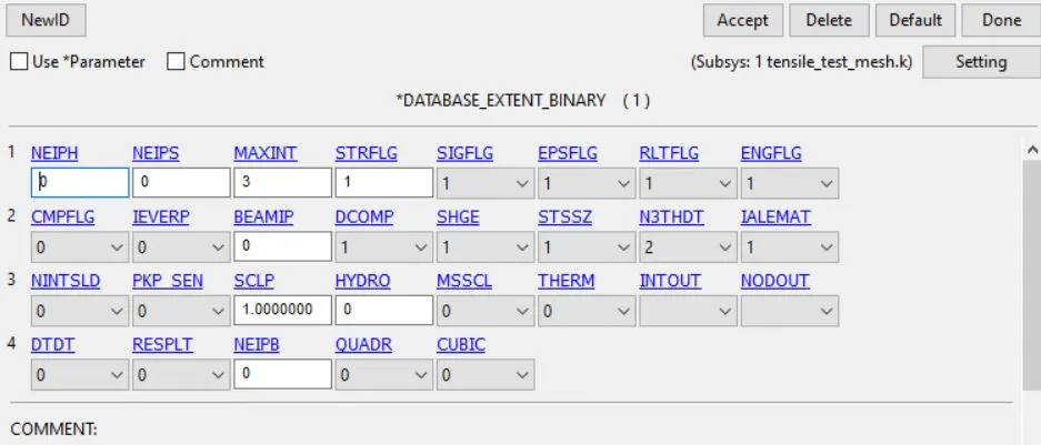
As it is a quaistatic process we need to do implicit run , so control implict_General, Control_Implicit_auto are activated,

IAUTO= 1, and IMFLAG= 1.

The simulation was run

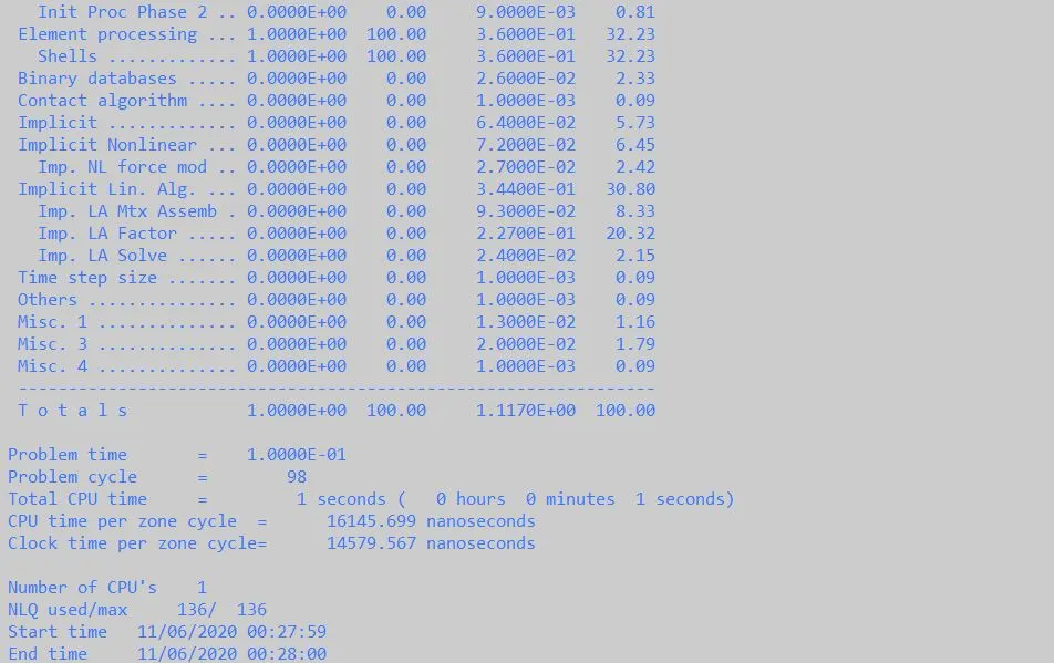
Post-processing:

The d3plot was loaded, and the effective stress and effective plastic strain values was plotted.

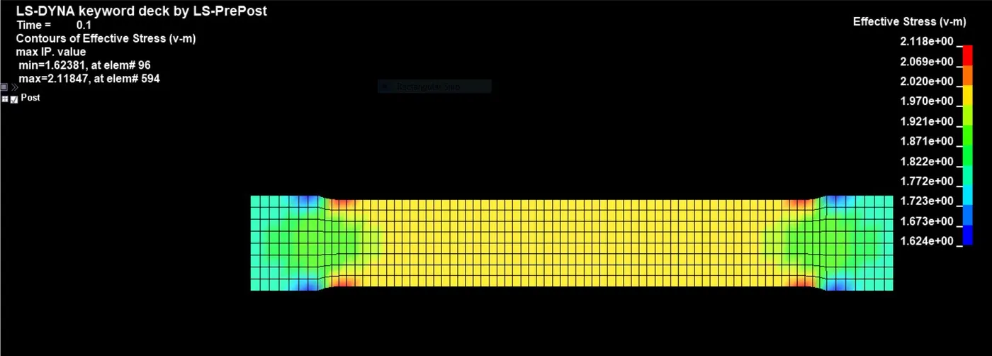
Fig: Effective stress plot at the highest stress value

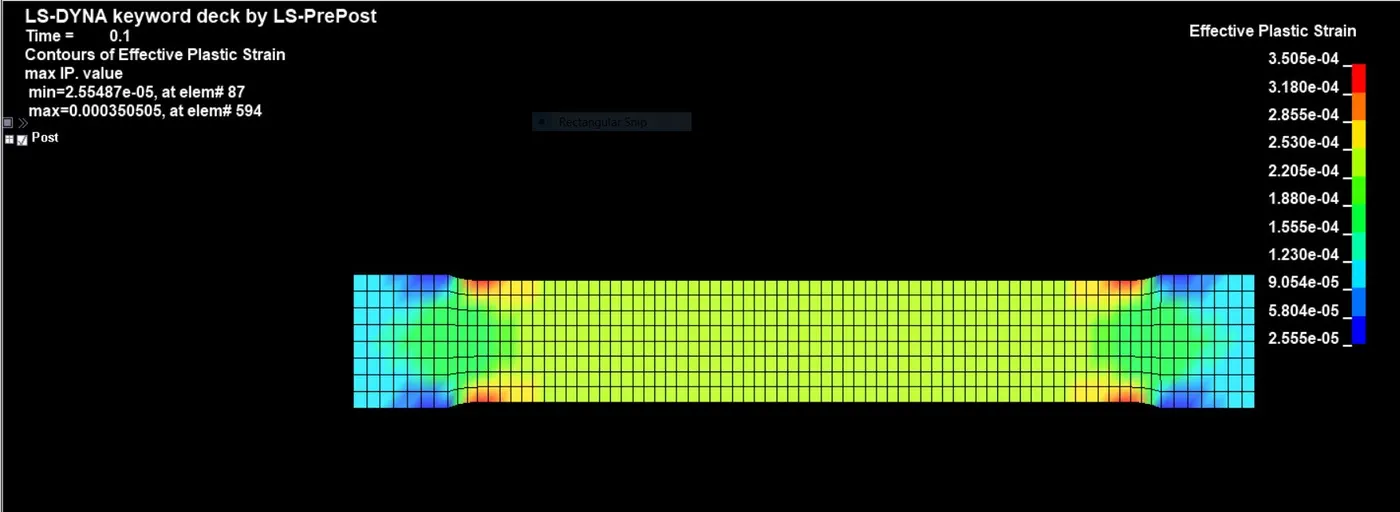
Fig: Effective plastic strain plot at the highest strain value

The history option in post processing is used to study the stress strain curve. Effective stress and effective plastic strain curves are plotted and then XY plot option is used where CROSS subsection is selected with the required axis to plot the effective stress and effective plastic strain plot.

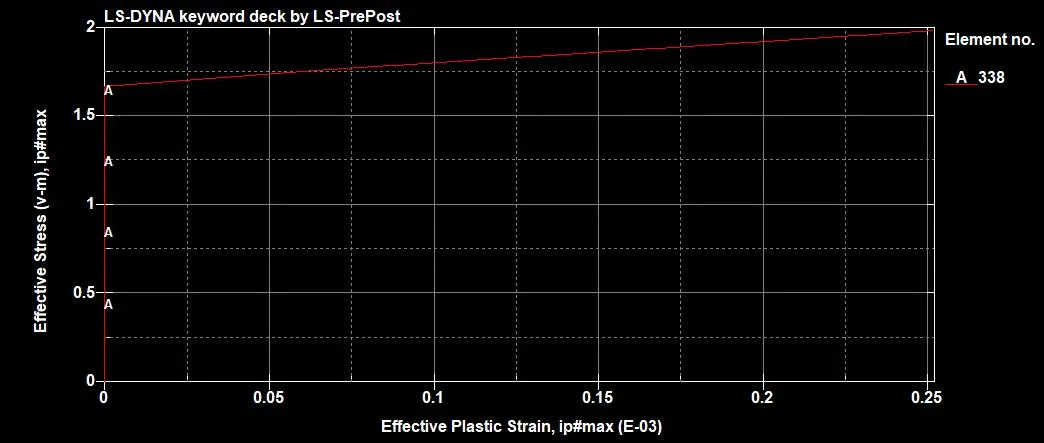
Conclusion : The curve was selected from the given picture, data points were extracted, cleaned and was implemented in MAT24 and used in simulation and the output curve can be compared with the input material curve for validation.