Week 9 - FVM Literature Review

Week 9 - FVM Literature Review

AIM:

1. What is the Finite Volume Method(FVM),
2. Write down the major differences between FDM & FVM.
3. Describe the need for interpolation schemes and flux limiters in FVM.
4. Use the 1D linear heat conduction equation as an example.

Finite Volume Method (FVM):

The Finite Volume Method (FVM) discretizes governing equations by conserving fluxes across control volumes, ensuring balance at each node. Ideal for fluid dynamics, it integrates differential equations over finite regions, converting them into algebraic forms. FVM excels in handling complex geometries and shock-capturing, preserving physical conservation laws effectively.

Write down the major differences between FDM & FVM:

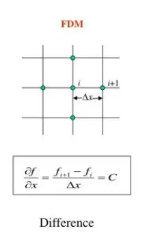
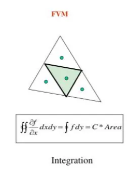
1. Discretization Approach – Finite Difference Method (FDM) approximates derivatives at discrete points using Taylor series, while Finite Volume Method (FVM) integrates conservation laws over control volumes, ensuring flux balance.

2. Conservation Property – FVM inherently preserves mass, momentum, and energy across control volumes, making it ideal for fluid dynamics, whereas FDM does not guarantee local conservation.

3. Geometric Flexibility – FVM easily adapts to complex, irregular grids and unstructured meshes, whereas FDM is typically confined to structured grids, limiting adaptability to intricate geometries.

4. Mathematical Formulation – FDM focuses on pointwise function approximations, whereas FVM derives algebraic equations from integral conservation laws, ensuring better physical accuracy.

5. Application Suitability – FDM is preferred for problems with simple domains and smooth solutions, while FVM excels in compressible flow, shock waves, and multiphase flow due to its flux-based formulation.

Describe the need for interpolation schemes and flux limiters in FVM.

In the Finite Volume Method (FVM), numerical accuracy and stability hinge on how values are estimated between computational nodes. This necessity drives the implementation of interpolation schemes and flux limiters to enhance solution precision, particularly for fluid flow and heat transfer problems.

Need for Interpolation Schemes

Since FVM operates on control volumes, variable values—such as velocity, pressure, or temperature—are often known only at discrete cell centers. To compute fluxes at cell faces, these values must be interpolated. Linear interpolation (central difference scheme) ensures second-order accuracy but can introduce numerical oscillations in high-gradient regions. Upwind schemes, which consider flow direction, improve stability but introduce numerical diffusion, leading to smeared solutions. More advanced schemes like QUICK (Quadratic Upstream Interpolation for Convective Kinematics) or MUSCL (Monotonic Upstream-Centered Scheme for Conservation Laws) strike a balance between accuracy and stability.

Need for Flux Limiters

When solving convection-dominated problems, sharp gradients such as shock waves or boundary layers can cause numerical oscillations if higher-order schemes are used indiscriminately. Flux limiters help prevent these by blending between high-order and low-order schemes, ensuring numerical stability while maintaining sharp solution features. TVD (Total Variation Diminishing) limiters, such as Van Leer, Superbee, and Minmod, are commonly used to eliminate spurious oscillations while preserving smooth transitions.

Thus, interpolation schemes and flux limiters are crucial in FVM to achieve accuracy, stability, and physical realism, especially in solving real-world aerospace and fluid mechanics problems.

1D Finite Volume Discretization of Heat Conduction
Governing Equation

The steady-state, one-dimensional heat conduction equation with an internal heat source is given as:

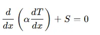
where T represents temperature, α denotes thermal diffusivity, and S is the source term. The temperatures at points A and B are specified as boundary conditions.

Discretization in Finite Volume Method (FVM)

To apply FVM, the domain is divided into control volumes centered around computational nodes. Each control volume extends between w (west face) and e (east face), enclosing a nodal point P. The fundamental principle in FVM is to integrate the governing equation over a control volume, ensuring flux balance across boundaries.

Using the divergence theorem, the diffusive flux leaving the east face minus that entering the west face is equated to the internal heat generation within the control volume:

$$A \left( \alpha \frac{dT}{dx} \Big|_e - \alpha \frac{dT}{dx} \Big|_w \right) + S \Delta V = 0$$

where A represents cross-sectional area, and ΔV denotes control volume size.

Central Differencing Approximation

For accurate representation, the temperature gradient at control volume interfaces is estimated using a central differencing scheme:

$${\left(\frac{dT}{dx}\right)}_e\approx \frac{T_E-T_P}{\delta x_{PE}},{\left(\frac{dT}{dx}\right)}_w\approx \frac{T_P-T_W}{\delta x_{W\mathrm{P}}}$$

Substituting these expressions into the discretized equation and rearranging terms yield a standard finite volume formulation:

$$a_P T_P = a_W T_W + a_E T_E + S_U$$​

where a_W, a_P, and a_E are coefficients ensuring conservation.

Interpolation Schemes in FVM

In FVM, estimating values at locations between computational nodes is essential for evaluating surface and volume integrals accurately. This requires interpolation schemes to approximate intermediate values.

First-Order Upwind Scheme

This method accounts for flow direction by using the upstream node's value. If flow velocity v > 0, the interface value is approximated using the left node:

$$\phi_{i+1/2} = \phi_i$$

If v < 0, the downstream node's value is used:

$$\phi_{i+1/2} = \phi_{i+1}$$​

This approach is stable but introduces numerical diffusion.

Backward and Forward Differencing

For cases where gradients need estimation, backward and forward differencing methods are used:

• Backward Differencing (when $v > 0$v>0):

$$I_c = v \frac{u_i - u_{i-1}}{\delta x}$$Ic​=vδxui​−ui−1​​

• Forward Differencing (when $v < 0$v<0):

$$I_c = v \frac{u_{i+1} - u_i}{\delta x}$$Ic​=vδxui+1​−ui​​

Taylor Series Expansion

Expanding function values at intermediate locations using Taylor series provides higher-order accuracy:

$$v u_{i+0.5} = v u_i + v \frac{\Delta x}{2} \left( \frac{\partial u}{\partial x} \right)_{i+0.5} + O(\Delta x^2)$$vui+0.5​=vui​+v2Δx​(∂x∂u​)i+0.5​+O(Δx2)

This introduces a numerical diffusion term, impacting accuracy.

Central Differencing Approximation

A second-order accurate scheme, central differencing linearly interpolates values between nodes L and R:

$${\varphi }_{i+1\mathrm{/}2}=\frac{{\varphi }_L+{\varphi }_R}{\mathrm{2}}$$

This scheme enhances accuracy but may cause oscillations in high-gradient regions.

QUICK Scheme (Quadratic Upwind Interpolation for Convective Kinematics)

The QUICK scheme provides higher accuracy by incorporating information from three adjacent nodes, making it suitable for convective transport problems.

---

Flux Limiters in FVM

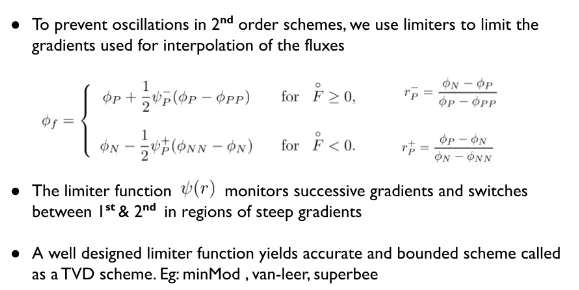
Higher-order schemes often lead to non-physical oscillations near sharp gradients. Flux limiters act as stabilizers by switching between low and high-order schemes depending on local solution behavior.

• In smooth regions, high-resolution schemes are retained for accuracy.
• Near discontinuities or shocks, limiters reduce oscillations by blending with lower-order upwind schemes.

Common flux limiters include Van Leer, Superbee, and Minmod, ensuring stability while preserving sharp solution transitions.

By combining appropriate interpolation schemes and flux limiters, FVM achieves numerical stability, accuracy, and conservation in solving heat conduction and other transport phenomena.

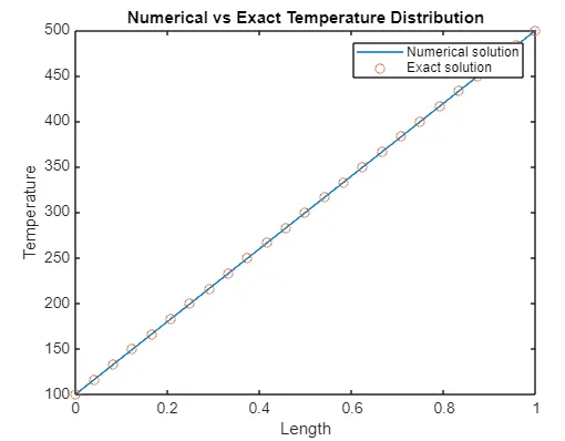
Case-1

The absence of a source term in the heat conduction equation

Matlab Code

% 1D heat conduction using finite volume method
% Steady state, no source term

% Constants
n = 25;
L = 1;
K = 1000;
Area = 1e-2;

% Discretization
x = linspace(0, L, n);
dx = x(2) - x(1);

% Boundary conditions
T = ones(1, n) * 100;
T(end) = 500;
T_exact = 400 * x + 100;

% Iterative solution
tol = 1e-7;
error = inf;
iter_number = 0;
while error > tol
    T_old = T;
    for i = 2:n-1
        a_p = 2 * K * Area / dx;
        a_e = K * Area / dx;
        a_w = K * Area / dx;
        T(i) = (a_w * T_old(i-1) + a_e * T_old(i+1)) / a_p;
    end
    error = max(abs(T_old - T));
    iter_number = iter_number + 1;
end

% Plotting
plot(x, T)
hold on
plot(x, T_exact, 'o')
title('Numerical vs Exact Temperature Distribution')
legend('Numerical solution', 'Exact solution')
ylabel('Temperature')
xlabel('Length')

Result

Case-2

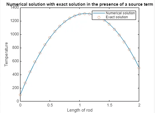
The Presence of a source term in the heat conduction equation

MATLAB CODE :

clear
close all
clc

% Parameters
n = 25;
L = 2;
x = linspace(0, L, n);
dx = x(2) - x(1);

% Initial and boundary conditions
T(1) = 100;
T(n) = 500;
T_old = T;

% Constants
K = 0.5;
Area = 1;
q = 1000;
source_term = q * Area * dx;

% Exact solution
T_exact = ((400 / L) + (500 / K) * (L - x)) .* x + 100;

% Iterative solution
error = inf;
tol = 1e-7;
while error > tol
    for i = 2:n-1
        a_p = 2 * K * Area / dx;
        a_e = K * Area / dx;
        a_w = K * Area / dx;
        T(i) = (a_w * T_old(i-1) + a_e * T_old(i+1) + source_term) / a_p;
    end
    error = max(abs(T_old - T));
    T_old = T;
end

% Plotting
figure;
plot(x, T)
hold on
plot(x, T_exact, 'o')
title('Numerical solution with exact solution in the presence of a source term')
legend('Numerical solution', 'Exact solution')
ylabel('Temperature')
xlabel('Length of rod')
pause(0.03)

RESULT :

Conclusion

The graph shows that increasing the number of nodes improves the accuracy of the numerical solution.