Challenge

Week 9 - FVM Literature Review

VVinodh Kumar Kg4 Nov 2020

FVM Literature Review:

The Finite volume method (FVM) is a widely used numerical technique.
The fundamental conservation property of the FVM makes it the preferable method in comparison to the other methods, i.e., FEM, and finite difference method (FDM).
Also, the FVM’s approach is comparable to the known numerical methods like FEM and FDM, which means that its evaluation of volumes is at discrete places over a meshed geometry.
Furthermore, the FVM transforms the set of partial differential equations into a system of linear algebraic equations.
Although the discrete approximation procedure in use in the FVM is distinctive, it also utilizes two basic steps.
Firstly, it transforms and integrates the PDEs into balance equations over an element.
The process incorporates the changing of the surface and volume integrals into discrete algebraic relations over elements as well as their surfaces using an integration quadrature of a specified order of accuracy.
This will result in a set of semi-discrete equations.
Secondly, in this next step, the interpolation profiles are chosen to estimate the variation of the variables within the element and relate the surface values of the variables to their cell values and thus transform the algebraic relations into algebraic equations.

In regards to the two steps in the FVM process, your approximation selection affects the overall accuracy of the subsequent numeric.

DIFFERENCE BETWEEN FVM & FDM:

Form of discretization based on the integral form of conservation equation.
In Finite difference Method we represent computitional domian as a set of parts.
However In Finite Volume Method we have the finitie volume bascially orbitary sgape volume within which the governing equation are solved.
FDM - The governing equation where as solved in a Point.
FVM - The equations are solved for a particular volume.
In FVM the conservation property Automatically Included in the equation infact in finitie different Method not.
The finitie volume method is a method for representing and evaluating Partial differential eqautions in the form of algebraic equations.
In the finite volume method, volume integrals in a partial differential equation that contain a divergence term are converted to surface integrals, using the divergence theorem.
These terms are then evaluated as fluxes at the surfaces of each finite volume.
Because the flux entering a given volume is identical to that leaving the adjacent volume, these methods are conservative.
The method is used in many computional filud dynamics packages.
"Finite volume" refers to the small volume surrounding each node point on a mesh.
Finite volume methods can be compared and contrasted with the finitie difference methods, which approximate derivatives using nodal values, or finitie difference methods, which create local approximations of a solution using local data, and construct a global approximation by stitching them together.
In contrast a finite volume method evaluates exact expressions for the average value of the solution over some volume, and uses this data to construct approximations of the solution within cells.

ADVANTAGES AND DISADVANTAGES OF FVM:

The FVM is a natural choice for solving CFD issues because the PDEs you have to resolve for CFD are conservation laws.
However, you can also use both FDM and FEM for CFD, as well.
The finite volume method is that it is easily formulated to allow for unstructured meshes.
The FVM’s most significant advantage is that it only needs to do flux evaluation for the cell boundaries.
Also, this is true for nonlinear issues as well, which, in turn, makes it an excellent choice for the handling of (non-linear) conservation laws.
The accuracy of the FVM, for example, close to a corner of interest, can be increased by refining the mesh around that corner, similar to the FEM.
However, unlike the FEM, the functions to estimate the solution is not easily made for higher-order.
Therefore, this is a disadvantage of the FVM versus the FEM.

Finite volume method for one-dimensional steady state diffusion

The finitie volume method in computational fluid dynamics is a discretization technique for partial differetial equations that arise from physical conservation laws.
These equations can be different in nature, e.g. elliptic, parabolic, or hyperbolic

General Transport equation can be defined as

where,
is density and is the conserved quantity.
is the Diffusion coefficient and S is the Source term.
is the Net rate of flow out of fluid element.
is Rate of increase of due to diffusion.
is Rate of increase of due to sources.

is Rate of increase of of fluid element(transient).

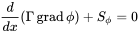
For one-dimensional, steady-state diffusion, General Transport equation reduces to:

or,

The following steps comprise the finite volume method for one-dimensional steady state diffusion -

STEP 1
Grid Generation

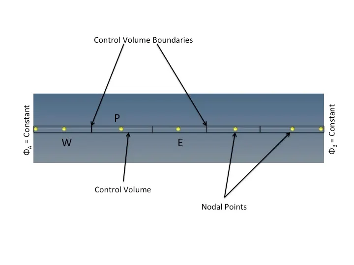
Divide the domain into equal parts of small domain.

Place nodal points at the center of each small domain.

Dividing small domains and assigning nodal points

Create control volumes using these nodal points.

Control volume and control volume & boundary faces

Create control volumes near the edges in such a way that the physical boundaries coincide with control volume boundaries (Figure 1).
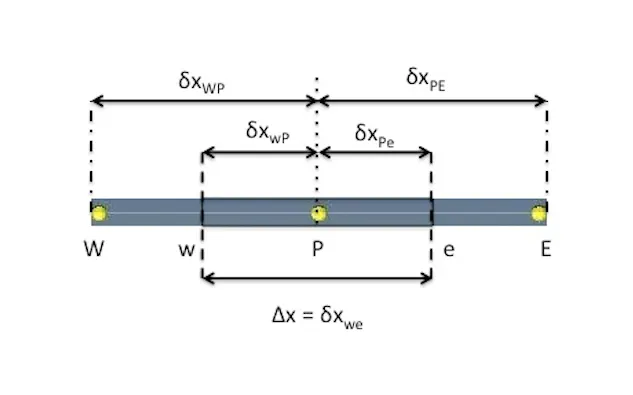
Assume a general nodal point 'P' for a general control volume.
Adjacent nodal points to the East and West are identified by E and W respectively.
The West-side face of the control volume is referred to by 'w' and the East-side control volume face by 'e'.

Steady state one-dimensional diffusion

The distance between WP, wP, Pe and PE are identified by,, and respectively.

STEP 2
DISCRETIZATION:

Control volume width

The crux of Finite volume method is to integrate the governing equation over each control volume.
Nodal points are used to discretize equations.
At nodal point P, the control volume integral is given

,

where

A -is Cross-sectional Area Cross Section Geometry of control volume face.

is Volume.

is average value of source S over the control volume.

It states that the difference between the diffusive flux Fick's laws of diffusion of through the east and west faces of some volume corresponds to the change in the quantity in that volume.
The diffusive coefficient of and are required in order to reach a useful conclusion.
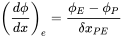
Central differencing technique is used to derive the diffusive coefficient of :

,

.

is calculated using the nodal point values

,
,

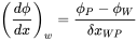In some practical situations, the source term can be linearized:

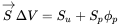Merging the above equations leads to

STEP 3:
Solution of equations

Discretized equation must be set up at each of the nodal points in order to solve the problem.
The resulting system of linear algebraic equations Linear Equation can then be solved to obtain at the nodal points.
The matrix of higher order can be solved in MATLAB.

INTERPOLATION:

Interpolation is the process of using points with known values or sample points to estimate values at other unknown points.
It can be used to predict unknown values for any geographic point data, such as elevation, rainfall, chemical concentrations, noise levels, and so on.

NEED FOR INTERPOLATION SCHEME IN FVM:

In FVM method we need to calculate the variables at th eparticular location other than computational nodes

Various Interpolation Schemes in FVM are:

FIRST ORDER UPWIND SCHEME:

In this scheme we need to define only one values from the upstream of cell centres.

SECOND ORDER UPWIND SCHEME:

In this scheme we need to define two values from the upstream cell centres.

QUADRATIC UPWIND INTERPOLATION SCHEME:

In this scheme we requires two upstream and one down stream cell centres.

CENTRAL DIFFERENCE SCHEME:

In this scheme we requires one upstream and one downstream value.

FORWARD DIFFERENCING SCHEME:

A forward difference is an expression of the form

Depending on the application, the spacing h may be variable or constant.

When omitted, h is taken to be 1:

Δ[ f ](x) = Δ₁[ f ](x).

we are getting information from the current point and the point of the Right hand side is called forward difference approximation.

BACK DIFFERENCE SCHEME:

A backward difference uses the function values at x and x − h, instead of the values at x + h and x:

we are getting information from the current point and the point of the left hand side is called forward difference approximation.

EXPLANATION:

Using this three types of finitie difference which we explained above

Seperately created function for

First_order_approximation(x , dx).
Second_order_approximation(x , dx).
Fourth_order_approximation(x , dx).

From the given equation

The Respective differencing, having know as a forward and central difference for the first two & for fourth order approximation we are using central difference.
In each one of them an output parameter is obtained respesenting the error difference according to the approximation and to the analytical derivative.
If it is first order method its taking information from one additional point.
If it is second order method its taking information from two additional points.
If it is fourth order method more information going to taken from the neighbouring points.

FLUX LIMITERS:

Flux limiters are used in high resolution schemes – numerical schemes used to solve problems in science and engineering, particularly fluid dynamics, described by Partial differential equations (PDE's).
They are used in high resolution schemes, such as the MUSCL scheme, to avoid the spurious oscillations (wiggles) that would otherwise occur with high order spatial discretization schemes due to shocks, discontinuities or sharp changes in the solution domain.
Use of flux limiters, together with an appropriate high resolution scheme, make the solutions total variation diminishing(TVD).
Note that flux limiters are also referred to as slope limiters because they both have the same mathematical form, and both have the effect of limiting the solution gradient near shocks or discontinuities.
In general, the term flux limiter is used when the limiter acts on system fluxes, and slope limiter is used when the limiter acts on system states (like pressure, velocity etc.)

NEED FOR FLUX LIMITERS IN FVM:

Interpolation schemes give good results.
In case of shock flow problem its disconitnuties, for that we need flux limiter.
The limiter function is constrained to be greater than pr equal to zero.
Therefore when the limiter is equal to zero the flux is represented by a low resolution scheme.
similarly when the limiter is equal to 1 it is represented by a high resolution scheme.

How its works:

The main idea behind the construction of flux limiter schemes is to limit the spatial derivatives to realistic values – for scientific and engineering problems this usually means physically realisable and meaningful values.
They are used in high resolution schemes for solving problems described by PDEs and only come into operation when sharp wave fronts are present.
For smoothly changing waves, the flux limiters do not operate and the spatial derivatives can be represented by higher order approximations without introducing spurious oscillations.
Consider the 1D semi discrete scheme below,

where, and represent edge fluxes for the ith cell.

If these edge fluxes can be represented by low and high resolution schemes, then a flux limiter can switch between these schemes depending upon the gradients close to the particular cell, as follows, ,

where

low resolution flux,

high resolution flux,

flux limiter function,

and r represents the ratio of successive gradients on the solution mesh, i.e.,

The limiter function is constrained to be greater than or equal to zero.

i.e., {\displaystyle \phi \ (r)\geq 0}

Therefore, when the limiter is equal to zero (sharp gradient, opposite slopes or zero gradient), the flux is represented by a low resolution scheme.
Similarly, when the limiter is equal to 1 (smooth solution), it is represented by a high resolution scheme.
The various limiters have differing switching characteristics and are selected according to the particular problem and solution scheme.
No particular limiter has been found to work well for all problems, and a particular choice is usually made on a trial and error basis.