FVM Literature Review
Objective
To describe the need for interpolation schemes and flux limiters in Finite Volume Method.
In computational fluid dynamics, three methods are commonly used for discretizing the PDE.
- Finite difference method
- Finite element method
- Finite volume method
Finite-Difference Method:
The finite-difference method is defined dimension per dimension this makes it easy to increase the “element order” to get higher-order accuracy. If you can fit the simulation in a rectangular or box shaped geometry using a regular grid, efficient implementations are much easier than for finite-element and finite-volume methods. Regular grids are useful for very-large-scale simulations on supercomputers often used in as mentioned before, meteorological, simological and astrophysical simulations.
With the finite-difference method, you may easily run into problems handling curved boundaries for the purpose of defining the boundary conditions. Boundary conditions are needed to truncate the computational domain. They represent communication with the surrounding world, which is the part that you do not want included in your simulation. If one can overcome the boundary condition problem on curved boundaries, the method gives very efficient and high quality results.
For computations that need high accuracy, the extra effort in making boundary-fitted meshes and the associated complications of such meshes for the implementation may be worth it. Examples include Formula 1 car computational-flulid-dynamic (CFD) simulations and space shuttle CPD simulations. The finite-difference method is more difficult to use for handling materials discontinuities. In addition, it does not lend itself for local grid refinement or anything similar to “adaptive mesh refinement”. This may be needed to resolve local rapid variations in solutions such as around a corner of a complex shape, described earlier
Finite Element Method:
One reason for the finite element methods success in multi-physics analysis is that it is a very general method. Solving the resulting equation systems are the same or very similar to well-know and efficient methods used for structural and electromagnetics analysis. Another reason for the method's success is that it makes it easy to “increase the order of the elements” so that the physics fields can be approximated very accurately. This typically corresponds to locally approximating the physics fields with polynomials of "higher order," such as second- and third-degree polynomials, or higher. This technique is often critical for example, in the case of accurate stress analysis.
If we consider the example of stress analysis, it is quite common that there are important stress concentrations close to some of the corners of a mechanical part. In this case, the finite-element method allows for two different ways of increasing the accuracy of the solution around this corner. One way is to increase the order of the elements, as described earlier. Another method is to locally refine the mesh close to that corner, the element density increases locally, The finer the mesh (i.e., more elements), the more accurate approximation one gets for the stress field around the corner of interest. Both techniques are used in finite-element software and are frequently made automatic from the user's perspective. This is known as "adaptive mesh refinement."
Another advantage with the finite-element method, which is particularly important for multi-physics analysis, is that you can combine different kinds of functions that approximate the solution within each element. This is called mixed formulations, This is important, for example, in the case of electromagnetic heating. The physics and mathematics require one type of function for the electromagnetic field and another type of function for beat transfer; they both need to be tightly coupled to get an accurate solution and for the solution to converge. Mixed formulations are straightforward to handle the finite-element method, but difficult or impossible with other methods.
The benefits with both the finite-element method and the finite-volume method are that curved and irregular CAD geometries are handled in a natural way.
However, the mathematics behind the finite-element method is quite advanced and thus the method requires mathematical expertise for its implementation. Implementations of finite-difference and finite-volume methods are comparatively straightforward.
For certain time-dependent simulations, one needs to use so-called explicit solvers for reasons of efficiency. Implementing such solver techniques is more difficult for the finite element method than for the finite-difference and finite-volume methods. However, this has successfully been commercialized in some cases, such as in crash simulations.
Finite volume method (FVM):
The finite volume method (FVM) is a method for representing and evaluating partial differential in the form of algebraic equations. In the finite volume method, volume integrals in a partial differential equation that contain a divergence term are converted to surface integrals, using the divergence theorem. These terms are then evaluated as fluxes at the surfaces of each finite volume. Because the flux entering a given volume is identical to that leaving the adjacent volume, these methods are conservative. Another advantage of the finite volume method is that it is easily formulated to allow for unstructured meshes. The method is used in many computational fluid dynamics packages. "Finite volume" refers to the small volume surrounding each node point on a mesh.
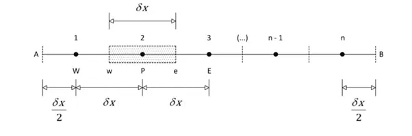
For example, consider steady state 1D linear heat conduction equation
`d/dx(Gamma*(dphi)/dx)+S_phi=0`
In Fig., n nodes are defined between the boundary temperatures. With the FVM, a general node P is defined at node 1, with node 1 and node 3 the west (W) and east (E) nodes of P, respectively. The control volume is bound by the west (w) and east (e) faces, which are placed at the midpoint between W and P, and P and E, respectively. To implement the FVM, Eq. 3 must be integrated over the control volume defined at P, which gives:
`int_(CV)d/dx(Gamma*(dphi)/dx)*dV+int_(CV)*S_phi*dV=(GammaA(dphi)/dx)_e-(GammaA(dphi)/dx)_omega+barS_(phi)DeltaV`
where A is the cross-sectional area of the control volume face, `DeltaV` is the volume and `barS_phi`is the average value of sources over control volume.
`barS_phi=S_u+S_(pphip)`
Interpolation schemes:
The evaluate the surface integrals and the volume integrals in the finite volume formulation, they require values at locations other than the computational nodes of the control volume. The values at these locations are obtained by using the interpolation formula. Hence interpolation schemes are important in Finite volume method.
Interpolation Methods in FVM:
Various possibilities for interpolation
- Upwind Interpolation Scheme
- Linear Interpolation Scheme
- Quadratic upwind Interpolation Scheme
- Hybrid, TVD and ENO Interpolation Scheme
Upwind Interpolation Scheme:
It is mainly used for the convection dominant problems. Velocity for a given point the direction of that velocity that determines the variables values used in interpolation process. In upwind scheme it makes use of nodes that are in the upstream of the given node.
It is used to calculate the approximate value of the variable(f) at the east face of the control volume, the equation is given by
`f_e={(fp if(V.n)_e>0),(f_E if (V.n)_e<0):}}`
where `f_P` is the point of the leftof face e
`f_E` is the point to the right of face e
(V.n) is Velocity vector
This scheme is almost like the forward difference approximation or a backward difference approximation based on the flow direction.
We know that when calculating gradience, we need to have those values bounded, so that they do not jump. Hence this approximation satisfies the boundness condition.
Linear Interpolation Scheme -
Linear interpolation is the method of generating new data points with a range of a discrete set of known data points.
`f_e=f_Elamda_e+f_P(1-lamda_e)`
where
`lamda_e=(x_e-x_p)/(x_E-x_P)`
The linear Interpolation scheme is same as the central difference formula that we considered for the first order derivative. So, this scheme is also known as the central difference scheme.
Generally, it is used to solve the integrated convection-diffusion equation.
It leads to a easy approximation for the evaluation of gradients that are required for evaluation of diffusive fluxes.
CDS is a second order accurate and may produce oscillatory solutions i.e here if the grid spacing is very large, we can find oscillatory solutions. It is basically a first order, as we refine the grid then accuracy is close to the second order.
Quadratic upwind Interpolation Scheme -
In CFD it is called as QUICK i.e. Quadratic Upstream Interpolation for Convective Kinematics
QUICK considers the second order derivative term into consideration and ignores the third order derivative term. Hence it is considered as third order accurate.
Now approximate the value of the variable at the face centre of the control volume by the quadratic interpolation by using the values at three nearest computational nodes i.e. 1 downstream node(D) and two upstream nodes(U, UU) respectively. The equation is given by
`f_e=f_U+g_1(f_D-f_U)+g_2(f_(UU)-f_U)`
where
`g_1=((x_e-x_U)(x_e-x_(UU)))/((x_D-x_U)(x_D-x_(UU))`
`g_2=((x_e-x_U)(x_e-x_(D)))/((x_(UU)-x_U)(x_(UU)-x_D)`
This scheme generally used to solve the convective-diffusion equations using the second order central difference for the diffusion term and for the convection term scheme is third order accurate in space and first order accurate in time.
Flux Limiter
Flux limiters used in high-resolution schemes, i.e. numerical schemes used to solve the problem in science and engineering, particularly fluid dynamics described by PDE. They are used in high-resolution schemes, namely the MUSCL scheme, to avoid spurious oscillation(wiggles) that would otherwise occur with high order spatial discretization schemes due to shocks, discontinuities, or sharp changes in the solution domain. The use of flux limiters, together with an appropriate high-resolution scheme, make the solution total variation diminishing (TVD).
Note that the flux limiters is also known as slope limiters both have the same mathematical form and also have the effect of limiting the solution gradient near shocks or discontinuities. In general, the flux limiter is used when the limiter acts on system states (Pressure, velocity)
`F(u_i+1/2)=f^(low)(i+1/2)-phi_(r_i)(f^(low)(i+1/2)-f^(high)(i+1/2))`
`F(u_i+1/2)=f^(low)(i+1/2)-phi_(r_(i-1))(f^(low)(i-1/2)-f^(high)(i-1/2))`
where `f^(low)`= low precision flux(1st order accurate)
`f^(high)`= high precision flux(highest order accurate)
`phi(r)`= flux limiter function,
r=`(u_i-u_(i-1))/(u_(i+1)-u_i)`
Need for Interpolation scheme and flux limiters FVM
1) The Guass or divergence theorem simply states that the outward flux of a vector field through a closed surface is equal to the volume integral of the divergence over the region inside the surface.
2) This theorem is a fundamental in the FVM it is used to convert the volume integral appearing in the governing equation into surface integrals.
3) The face value appearing in the convective and diffusive fluxes must be computed by some form of interpolation from the centroid value of the control volume at both sides of the face.
4)After spacial discretization, we can proceed win the temporal discretization. By proceeding in this way, we are using the method of lines (MOL).
5) The main advantage of the MOL method is that allows us to select numerical approximations of different accuracy for the spatial and temporal terms Each term be treated differently to yield different accuracies.
6) Nearly all flows in nature and industrial applications are unsteady (also known as transient or time dependent)
Unsteadiness is due to
- Instabilities
- Non- equilibrium initial conditions
- Time dependent boundary conditions
- Source term
- Chemical reactions
- Moving or deforming bodies
- Turbulence
- Buoyancy
- Convection
- Multiple phases
Steady Simulations vs Unsteady Simulations
1) The steady simulation requires less computational power than unsteady simulations.
2) They are also so much faster than unsteady simulations
3) But sometimes they do not converge to the right solution
4) They are easier to post-process and analyse
We can use the solution of an unconverted steady simulation as initial conditions for unsteady simulations.
Remember, steady simulation is not time accurate therefore we cannot use them to compute temporal statistics or compute the shedding frequency.
Following are the plots for 1D linear convection equation
where, n= Grid points.
For n=20
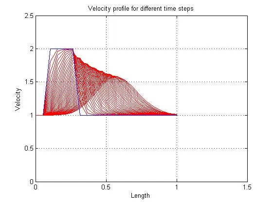
In the plot where n=20, there is a drastic decrease in the velocity profile
the amplitude of the velocity profile keeps decreasing with length
The minimum velocity is approximately is 1.6 to 1.7 m/s
For n = 40
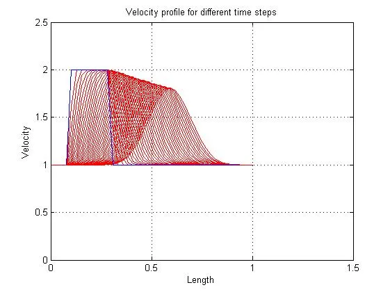
In the plot where n=40, there is a significant decrease in the velocity profile
the amplitude of the velocity profile keeps decreasing with length
The minimum velocity is approximately is 1.7 to 1.8 m/s
For n = 80
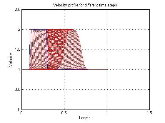
In this plot where n=80 there is a gradual decrease in the velocity profile, the change in the velocity profile with respect to length is not a major change Hence the amplitude is almost constant.
The min and max velocity very close to 2 m/s
For n = 160
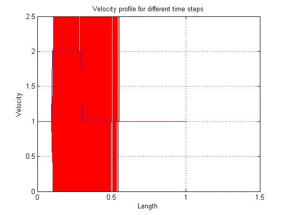
In this fig,
There is a disturbance in velocity profile and there is a blow-up indeed, it is noticed that ripple formed in the plot making it unstable. The velocity profile gives an unstable graph.