Week 9 - FVM Literature Review
Aim: FVM Literature Review.
Objective
- What is Finite Volume Method(FVM)
- Write down the major differences between FDM & FVM.
- Describe the need for interpolation schemes and flux limiters in FVM.
Description (use Versteeg as a reference)
The finite volume approach is what?
The finite volume method (FVM) is a particular instance of the finite difference method (FD), which is one of three separate numerical solution approaches.
This algorithm includes integrating the governing equations across all of the domain's finite control volumes
the algebraic equations that correspond to the integral equations.
The algebraic equations are solved iteratively.
The FVM differs from all other CFD approaches in that the control volume integration produces statements that explain the precise conservation of each finite cell's characteristics, establishing a direct link between the physics and the numerical procedure. Compared to the FEM and spectral approaches, this makes concepts simpler to understand. The following is an example of how the numerical method/physics may be expressed:
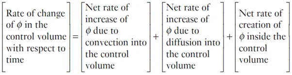
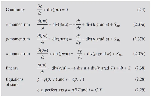
conveniently condensed into the following form via a general variable phi.
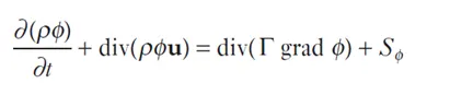
The above equation is called the transport equation for property phi. The key step in finite volume methods is to provide an integral form of the above equation over a three-dimensional control volume, given below.

After a suitable reordering of integrating/differentiation and using Gauss Theroem which states
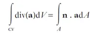
The resulting integral form can then be re-cast as below

This can be read as follows
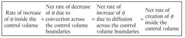
Major Difference between FDM and FVM
Since the former consists of algebraic equations approximating the derivative and the latter of algebraic equations approximating the integrals/fluxes, the form of the equations to be solved differs between FDM and FVM.
Finite difference techniques are often limited to grids with structure. This is because the Taylor expansion techniques call for holding the values of the first two of the three spatial components constant while building the Taylor expansion on the third component.
The use of transformation/mapping techniques for coordinate transformations is a workaround to allow the study of unstructured grids using the FDM.
Because the integral form of the equations is utilised in FVM, it is simple to handle unstructured grids because it enables the physical quantities to be preserved (and so monitored) both at the level of the finite cell and over the entire domain.
Planned Interpolations
We need to take into consideration how convection affects the way the carried material diffuses when we analyse fluid movement. We may use the steady state convection-diffusion equation, which is derived from the transport equation previously illustrated, as an example.
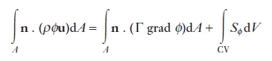
This crucial difference presents problems in calculating the convective fluxes across the boundary control faces.
It has been shown that using the central differing scheme is inadequate for describing the flow of convective-diffusive phenomena. For example, one of the major disadvantages of this scheme is the ability to identify flow direction.
Therefore, the properties of discretisation schemes are evaluated to ascertain their suitability via the following:
- Conservativeness
- Boundedness
- Transportability
Thus, alternative discretisation schemes have been developed to circumvent the weakness of central differencing schemes using the above mentioned properties.
- Upwind differencing schemes
- Hybrid differencing schemes
- Power law scheme
The three aforementioned systems have the drawback that, although being stable and adhering to the transportability criteria, they are only first order accurate, rendering them susceptible to numerical diffusion errors. Therefore, higher order differencing techniques are taken into consideration, including but not limited to
- QUICK (quadratic upstream interpolation for convective kinetics)
- TVD (total variation diminishing)