Finite Volume Method Literature Review

Finite Volume Method (FVM):

The Finite Volume Method (FVM) is a discretization method for the approximation of a single or a system of partial differential equations expressing the conservation, or balance, of one or more quantities. These partial differential equations (PDEs) are often called conservation laws; they may be of different natures, e.g. elliptic, parabolic or hyperbolic, and they are used as models in a wide number of fields. They describe the relations between partial derivatives of unknown fields such as temperature, concentration, pressure, density, etc. with respect to variables within the domain (space, time,...) under consideration.

As in the finite element method, a mesh is constructed, which consists of a partition of the domain where the space variable lives. The elements of the mesh are called control volumes. The integration of the PDE over each control volume results in a balanced equation. The set of balance equations is then discretized with respect to a set of discrete unknowns.

In this method, volume integrals in a partial differential equation that contain a divergence term are converted to surface integrals, using the divergence theorem. These terms are then evaluated as fluxes at the surfaces of each finite volume. Because the flux entering a given volume is identical to that leaving the adjacent volume, these methods are conservative. Another advantage of the finite volume method is used in many computational fluid dynamics packages.

"Finite volume" refers to the small volume surrounding each node point on a mesh which can be seen below:

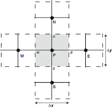
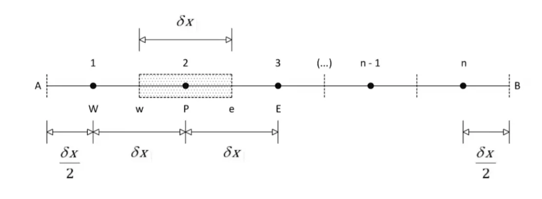
In the above figure, P is the current node and W is the node adjacent to the west of node P & E is the node adjacent to the east of node P. w & e are the starting points of control volume of the west and east side respectively. This pattern is also followed for north and south adjacent points and control volumes.

For example, consider steady-state 1D linear heat conduction equation:

`d/dx(Gamma.(dphi)/(dx))+S_(phi)=0`

In Fig., 𝑛 nodes are defined between the boundary temperatures. With the FVM, a general node 𝑃 is defined at node 1, with node 1 and node 3 the west (𝑊) and east (𝐸) nodes of 𝑃, respectively. The control volume is bound by the west (𝑤) and east (𝑒) faces, which are placed at the midpoint between 𝑊 and 𝑃, and 𝑃 and 𝐸, respectively. To implement the FVM, Eq. 3 must be integrated over the control volume defined
at 𝑃, which gives:

`int_(CV)d/dx(Gamma*(dphi)/(dx))*dV+int_(CV)S_phi*dV=(Gamma*A*(dphi)/(dx))_e-(Gamma*A*(dphi)/(dx))_w+S_phi*DeltaV`

where A is the crossectional area of the control volume face, `DeltaV` is the volume and `S_phi` is the average value of sources over control volume.

`S_phi=S_u+S_p*phi_p`

Major differences between FDM & FVM:

A finite difference method discretization is based upon the differential form of the PDE to be solved. Each derivative is replaced with an approximate difference formula. The computational domain is usually divided into hexahedral cells and the solution will be obtained at each nodal point. The FDM is easiest to understand when the physical grid is Cartesian, but through the use of curvilinear transforms the method can be extended to domains that are not easily represented by brick-shaped elements. The discretization results in a system of the equation of the variable at nodal points, and once a solution is found, then we have a discrete representation of the solution.

The finite volume method is a method for representing and evaluating partial differential equations in the form of algebraic equations. In the finite volume method, volume integrals in a partial differential equation that contain a divergence term are converted to surface integrals, using the divergence theorem. Useful for problems with body-fitted coordinate systems.

So between a differential and an integral scheme (integral scheme scores in terms of error). Differential schemes are faster and error can be minimized if we have regular grids (squares and rectangles). Integral schemes are slightly slower but score over FDM when the mesh is irregular.

Most commercial software like FLUENT is either FVM or FEM whereas FDM is a very popular method in academic circles.

Need for Interpolation:

Interpolation is a process to estimate the values at unknown points by using the points with a known value and sample points on either side of the computational node. In FVM, interpolation schemes are used to find values of volume integrals required at the points other than nodes.

The Guass or divergence theorem simply states that the outward flux of a vector field through a closed surface is equal to the volume integral of the divergence over the region inside the surface. This theorem is fundamental in the FVM, it is used to convert the volume integrals appearing in the governing equation into surface integrals.

The face values appearing in the convective and diffusive fluxes have to be computed by some form of interpolation from the centroid values of the control volume at both sides of the face. After spacial discretization, we can proceed with the temporal discretization. By proceeding in this way we are using the method of lines (MOL). The main advantage of the MOL method is that it allows us to select numerical approximations of different accuracy for the spatial and temporal terms. Each term can be treated differently to yield different accuracies. Nearly all flows in nature and industrial applications are unsteady (also known as transient or time-dependent).

Various Interpolation Scheme:

1. Upwind interpolation scheme
2. Linear interpolation scheme
3. Quadratic upwind interpolation scheme
4. Hybrid interpolation scheme
5. Total Variation Diminishing scheme (TVD)
6. Essentially Non-Oscillatory interpolation scheme (ENO)

1. Upwind interpolation scheme:

This scheme is generally used for convection dominated problems. In upwind differencing scheme, the flow direction is taken into account when calculating value at a cell. The convected value of `varphi` at a cell face is taken to be equal to the value at the upstream node.

When the flow is in the positive direction, `U_w>0,U_e>0text( )(F_w>0,F_e>0),` the upwind scheme sets as:

`phi_w=phi_Wtext( and )phi_e=phi_P`

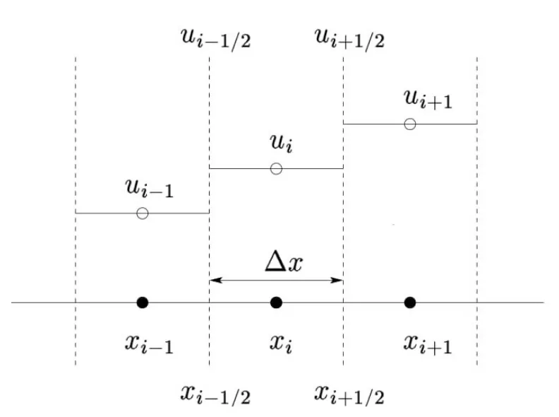
The upwind scheme for approximating the value of a variable f at the east face of a control volume is given by:

`f_e={(f_p if,(v*n)_e,>,0),(f_E if,(v*n)_e,<,0):}`

2. Linear interpolation:

To approximate the values of variables at control volume face Centre by linear interpolation of the values at two nearest computational nodes. This is equivalent to the use of the central difference scheme of first order derivatives, and it is also known as the Central difference scheme. This also leads to very simple approximation of evaluation of gradients required for evaluation of diffusive fluxes. the relation is given as follows:

`f_e=f_Elambda_e+f_p(1-lambda_e)text( where )lambda_e=(x_e-x_p)/(x_E-x_p)`

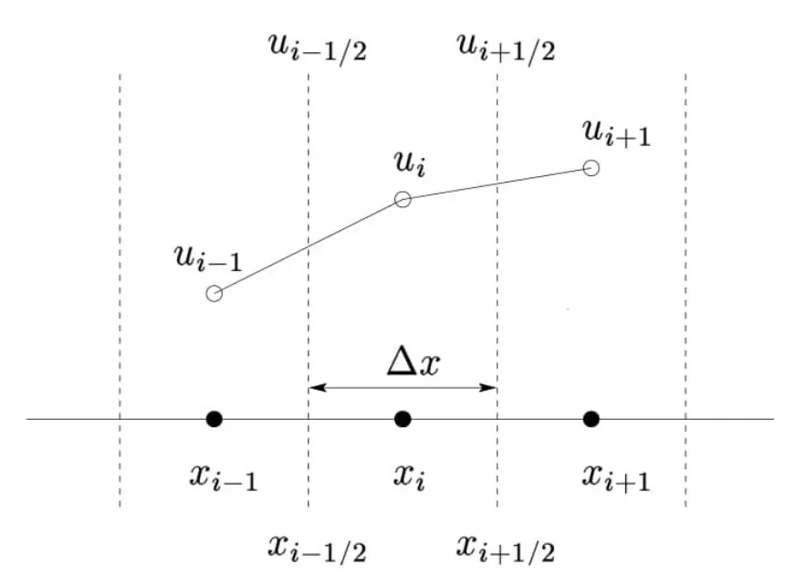
The approximation is second-order accurate. It is the simplest most widely used in interpolation for the evaluation of gradients required for the evaluation of diffusive fluxes.

3. Quadratic upwind interpolation scheme (QUICK):

This approximates the value of a variable at the control volume face centre by quadratic interpolation of the values at 3 nearest computational nodes ( one downstream node, D and to upstream nodes, U). It is third-order accurate for both uniform and nonuniform grids.

`f_e=f_U+g_1(f_D - f_U)+g_2(f_(UU)-f_u)`

`g_1=((x_e-x_U)(x_e-x_(UU)))/((x_D-x_U)(x_D-x_(UU)))`

`g_1=((x_e-x_U)(x_e-x_(D)))/((x_(UU)-x_D)(x_(UU)-x_(U)))`

The relation obtained is:

`phi_e=6/8phi_c+3/8phi_D-1/8phi_(UU)`

4. hybrid Interpolation Scheme:

It is the blend of CDS and UDS scheme, based on Peclet number.

`f_e=gammaf_(CDS)+(1-gamma)f_(UDS)`

5. Total Variation Diminishing Scheme:

`f_e=f_p+1/2psi(r)(f_E-f_p)`

where `psi` is the flux limiter.

FLUX LIMITERS:

For convective fluid flow, it is observed that the low order schemes are usually stable but quite dissipative in nature around the points of discontinuity for shocks, while the higher-order schemes are unstable in nature and show oscillations in the vicinity of discontinuity or shocks.

Highly accurate and oscillation free spins are known as high-resolution schemes.

Flux limiter functions are used to fine-tune the higher order and lower order scheme in a way that the resulting scheme gives a higher-order accuracy in the smooth region of the flow and maintains the first-order accuracy in the vicinity of shocks and discontinuities. For such a scheme TVD scheme is employed.

`F(u_(i+1/2))=f_(i+1/2)^(low)-phi(r_i)(f_(i+1/2)^(low)-f_(i+1/2)^(high))`

`F(u_(i+1/2))=f_(i-1/2)^(low)-phi(r_i-1)(f_(i-1/2)^(low)-f_(i-1/2)^(high))`

where,

`f^(low)=text( Low precission flux (1st order accurate))`

`f^(high)=text( High precission flux (Highest order accurate))`

`phi(r) = text( Flux limiter function where, )r=(u_i-u_(i-1))/(u_(i+1)-u_i)`