Simulation of a 1D Super-sonic nozzle flow simulation using MacorMack's Method
Objective: Primary objective of this project is to simulate flow inside a supersonic nozzle with 2nd order accuracy. To achieve this level of accuracy and to minimize the calculations involved, a commonly used technique called MacCormack's Method is used. This method uses the finite difference method to achieve 2nd order accuracy without involving 2nd order derivative which reduces mathematical complexity.
Reference: All the below formulation and calculations are done by referring to a book "Computational Fluid Dynamics" written by John D. Anderson, a digital copy of this book can be found on this link: Computational Fluid Dynamics by John D. Anderson
Problem description:
(NOTE: All the problem specification and formula derivation are done according to chapter 7 of the above-mentioned book, kindly refer to this book if u have any doubts regarding the formulation of the problem or governing equation derived)
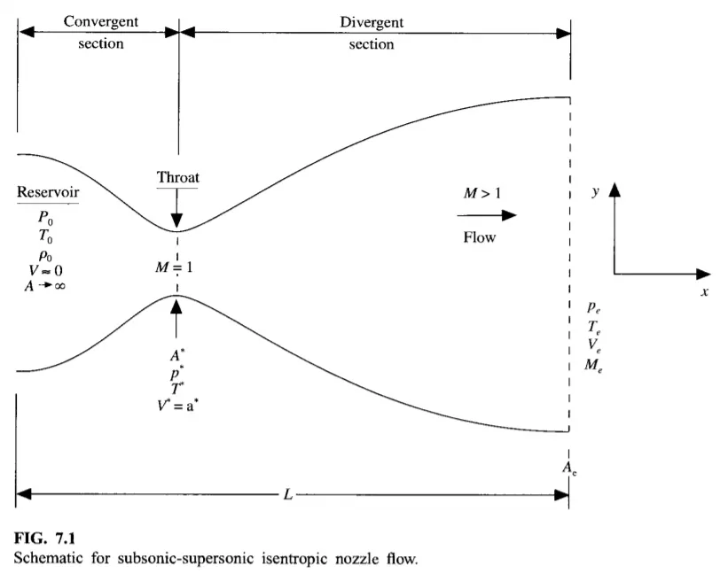
An isentropic flow through a convergent-divergent nozzle as sketched in Fig.7.1. The flow at the inlet to the nozzle comes from a reservoir where the pressure and temperature are denoted by `p_0` and `T_0`, respectively. The cross-sectional area of the reservoir is large (theoretically, `A rarr oo`), and hence the velocity is very small (`Vrarr0`), Thus, `p_0` and `T_0` are total pressure and total temperature, respectively. The flow expands isentropically to supersonic speeds at the nozzle exit, where the exit pressure, temperature, velocity, and Mach number are denoted by `p_e,T_e,V_e text( and ) M_e`, respectively.
The flow is locally subsonic in the convergent section of the nozzle, sonic at the throat (min. area), and supersonic at the divergent section.
Area of the nozzle changes as a function of distance along with the nozzle, `x`, and therefore in reality the flow field is two-dimensional, we make the assumption that the flow properties vary only with `x`. Such flow is defined as quasi-one-dimensional flow.
Governing equations:
Continuity equation: `rho_1V_1A_1=rho_2V_2A_2` ...............(1)
Momentum equation: `rho_1A_1+rho_1V_1^2A_1+int_(A_1)^(A_2)(rho*dA)=rho_2A_2+rho_2V_2^2A_2` ...............(2)
Energy equation: `h_1+(V_1^2)/2=h_2+(V_2^2)/2` ...............(3)
Non-dimensionalization:
Returning to Fig.7.1, where the reservoir temperatures and density are denoted by `T_0` and `rho_0`, respectively, we define the nondimensional temperature and density, respectively, as
`T'=T/T_0` `rho'=rho/rho_0`
letting L denote length of the nozzle, `x'=x/L`
speed of sound in the reservoir as, `a_0=sqrt(gammaRT_0)`
dimensionless velocity as, `V'=V/a_0`
dimensionless time as, `t'=t/(L/a_0)`
dimensionless area as, `A'=A/A^*`
where `A^**` is the sonic throat area
Nozzle shape:
Parabolic area distribution is given by:
`text( )A=1+2.2(x+1.5)^2 text( )0<=x<=3`
Non-Conservation form equations:
Continuity equation: `(delrho')/(delt')=-rho'*(delV')/(delx')-rho'V'(del(lnA'))/(delx')-V'(delrho')/(delx")` ...................(4)
Momentum equation: `(delV')/(delt')=-V'(delV')/(delx')-(1/gamma)*((delT')/(delx')+(T')/(rho')*(delrho')/(delx'))` ...................(5)
Energy equation: `(delT')/(delt')=-V'*(delT')/(delx')-(gamma-1)*T'*[(delV')/(delx')+V'(del(lnA'))/(delx')]` ...................(6)
Initial conditions:
`text( at t=0 ){(rho,=,1-0.3146x),(T,=,1-0.2314x),(V,=,(0.1+1.09x)T^(1/2)):}`
Boundary conditions:
At start:
`text( )V_1=2*V_2-V_3`
`text( Fixed, independent of time ) {(rho_1,=,1.0),(T_1,=,1.0):}`
At end:
`V_N=2*V_(N-1)-V_(N-2)`
`rho_N=2*rho_(N-1)-rho_(N-2)`
`T_N=2*T_(N-1)-T_(N-2)`
Conservation form equations:
Continuity equation: `(del(rho'A'))/(delt')+(del(rho'A'V'))/(delx')=0` ...................(7)
Momentum equation: `(del(rho'A'V'))/(delt')+(del[rho'A'V'^2+(1/gamma)rho'A'])/(delx')=1/gamma rho'(delA')/(delx')` ...................(8)
Energy equation: `(del[rho'((e')/(gamma-1)+gamma/2V'^2)A'])/(delt')+(del[rho'((e')/(gamma-1)+gamma/2V'^2)V'A'+rho'A'V'])/(delx')=0` ...................(9)
Let us define the elements of the solutions vector U, the flux vector F, and the source term J as follows:
`U_1=rho'A'`
`U_2=rho'A'V'`
`U_3=rho'((e')/(gamma-1)+gamma/2V'^2)A'`
`F_1=rho'A'V'`
`F_2=rho'A'V'^2+1/gammarho'A'`
`F_3=rho'((e')/(gamma-1)+gamma/2V')V'A'+rho'A'V'`
`J_2=1/gammarho'(delA')/(delx')`
These equations can be related as bellow:
`(delU_1)/(delt')=-(delF_1)/(delx')`
`(delU_2)/(delt')=-(delF_2)/(delx')+J_2`
`(delU_3)/(delt')=-(delF_3)/(delx')`
The pure form of the flux and source terms:
`F_1=U_2`
`F_2=(U_2^2)/(U_1)+(gamma-1)/(gamma)(U_3-gamma/2(U_2^2)/(U_1))`
`F_3=gamma(U_2U_3)/(U_1)-(gamma(gamma-1))/(2)U_2^3/U_1^2`
`J_2=(gamma-1)/(gamma)(U_3-gamma/2U_2^3/U_1^2)(del(lnA'))/(delx')`
Dimensionless primitive variables can be calculated as follows:
`rho'=U_1/(A')` `V'=U_2/U_1`
`p'=rho'T'` `T'=e'=(gamma-1)(U_3/U_2-gamma/2V'^2)`
Initial conditions:
`text(For ) 0<=x'<=0.5text( ){(rho',=,1.0),(T',=,1.0):}`
`text(For ) 0.5<=x'<=1.5text( ){(rho',=,1.0-0.366(x'-0.5)),(T',=,1.0-0.167(x'-0.5)):}`
`text(For ) 1.5<=x'<=3.5text( ){(rho',=,0.634-0.3879(x'-1.5)),(T',=,0.833-0.3507(x'-1.5)):}`
`text( )U_1=rho'A'`
`text( )U_2=rho'A'V' text( )U_2=0.59`
`text( )U_3=rho'((e')/(gamma-1)+gamma/2V'^2)A' text( where )e'=T'`
`text( )V'=U_2/(rho'A')=0.59/(rho'A'`
Value of `U_2` is selected as 0.59 as it is closest to the analytical value.
Boundary conditions:
At start:
`(U_1)_((i=1))=(rho'A')_((i=1))=A'_((i=1))=text(fixed value)`
`(U_2)_((i=1))=2*(U_2)_((i=2))-(U_2)_((i=3))` `U_3=U_1((T')/(gamma-1)+gamma/2V'^2)`
At end:
`(U_1)_N=2*(U_1)_(N-1)-(U_1)_(N-2)`
`(U_2)_N=2*(U_2)_(N-1)-(U_2)_(N-2)`
`(U_3)_N=2*(U_3)_(N-1)-(U_3)_(N-2)`
MacorMack's Technique:
For instance, assume we are calculating the continuity equation.
The first step in the Macromack procedure is to find predictor value which uses forward marching for the taken equation. Which will be:
`(delrho)/(delt)=-rho*(V_(i+1)-V_i)/(delx)-rhoV*(lnA_(i+1)-lnA_i)/(delx)-V*(rho_(i+1)-rho_i)/(delx)`
similar procedure is done to the momentum and energy equation.
Next step is to update all the three parameters given as boundary conditions for the next time step which can be done as:
`rho^(t+delt)=rho^t+((delrho^t)/(delt)*delt)`
where density derivative is the one which obtained in the previous step.
The next step is corrector step which has to be done for the three governing equations. In this backward/rearward difference must be used. So corrector step for density derivative can be calculated as:
`(delrho)/(delt)=-rho*(V_(i)-V_(i-1))/(delx)-rhoV*(lnA_(i)-lnA_(i-1))/(delx)-V*(rho_(i)-rho_(i-1))/(delx)`
and a similar procedure can be followed for velocity and temperature as well.
Now the derivatives of the parameters obtained from the corrector and predictor value should be averaged and then it should be updated in the next step. Density derivative can be done as:
`((delrho)/(delt))_(avg)=0.5*[((delrho)/(delt))_(text(predictor))+((delrho)/(delt))_(text(corrector))]`
where predictor and corrector derivative values are obtained from the previous two steps.
The last step is to update the obtained average value of derivative with the value at beginning of time step by multiplying with `delt`.
`rho^(t+delt)=rho^t+((delrho)/(delt))_(avg)*delt`
This step will be repeated until it reaches a certain convergence.
The same procedure can be used for conservative form as well just by replacing the governing equations and following the same steps.
The main Advantage of using the MacroMack technique is that it will be using forward difference for predictor step and backward difference for corrector step. Both forward and backward difference methods are first-order approximation which just uses first-order differential equations. If we go for a second-order central difference scheme it will be having second-order differential equations which take a lot of time for computation. Hence as an order of central difference goes up gradually time for solving too will take so long. So, it doesn’t mean the use of MacCormack technique (first-order) will yield poor results. Since it's taking corrector (backward method) and predictor(forward method) for computing and this average value is updated at each time step it will be accurate like second-order technique but it will take less amount of time than second-order because of a lower-order partial differential equation.
Time-step calculation:
The most important factor of any simulation is the stability of the solution. It highly depends on the value of time step increments. In this particular case time step can be calculated as:
`del t=CFL*(delx)/(a+V)`
where CFL is Courant Friedrichs Lowry (CFL) number which determines the stability highly. Usually, the value of CFL must be less than 1, or else the solution will blow up as seen in previous challenges. Now, deltax is the distance between each node, a is the velocity of sound and V is local velocity. But velocity value will be changing at each and every point in this challenge so, the minimum value from the above step is used
as time step calculation of the solution. It's noted that for CFL above one solution isn't stable. As well CFL is 0.9 it takes a lot of iteration than usual to converge. Hence 0.5 is idle CFL number for this challenge.
Programming:
The program is divide into 3 parts, part 1 is the main body where the initial conditions and boundary layer and other details which are required to solve the governing equations are calculated and passed tot respective functions. 2nd part is defined as a non-conservative method to solve the problem and the last part is defined as a constructive method to solve the problem.
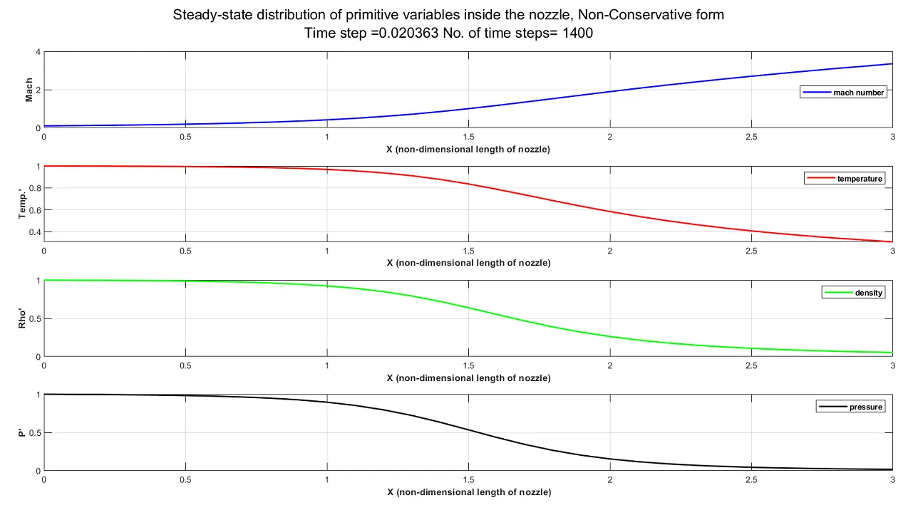
Figure 1: Steady-state distribution of primitive variables inside the nozzle
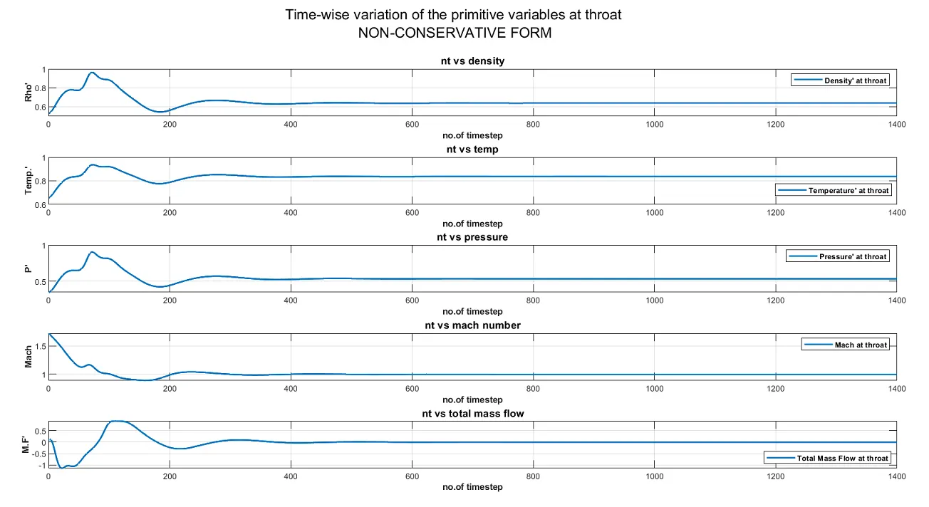
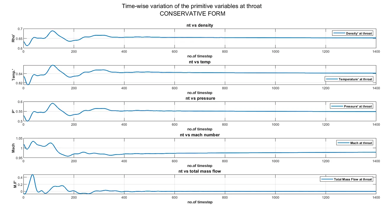
Figure 2: Time-wise variation of the primitive variables
Figure 3: Variation of Mass flow rate distribution inside the nozzle at different time steps during the time-marching process
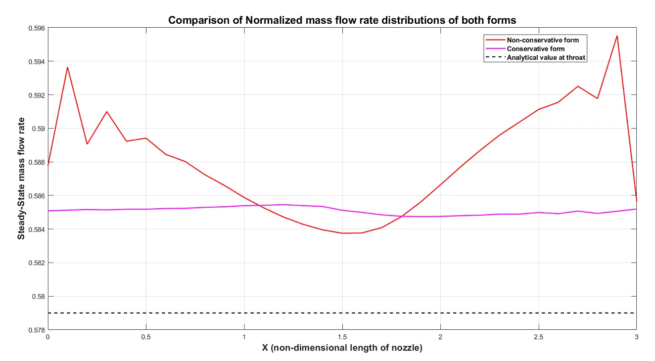
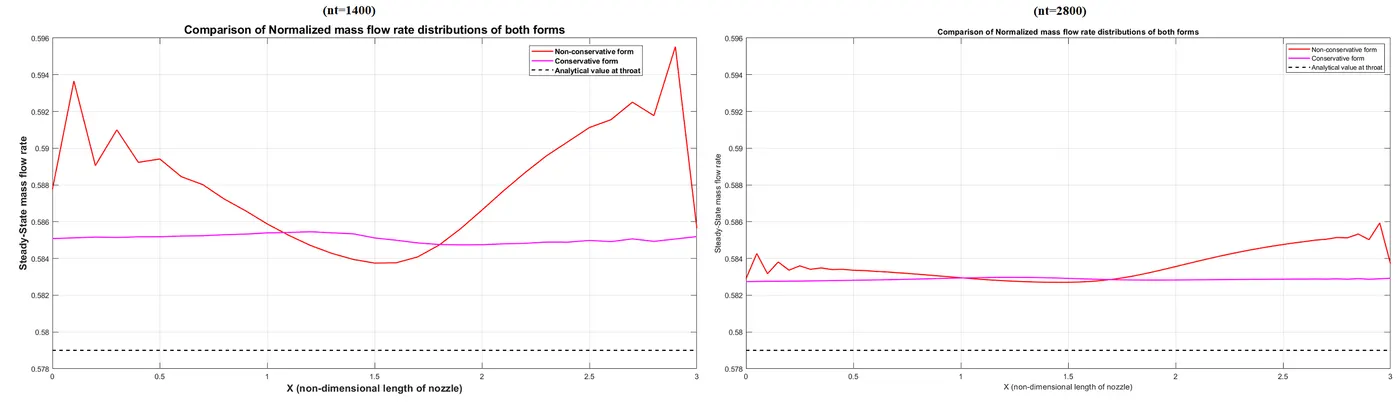
Figure 4: Comparison of Normalized mass flow rate distributions of both forms
Main Program:
clear all
close all
clc
%inputs
n=31;%number of grid points, case 1
x=linspace(0,3,n);
dx=x(2)-x(1);
c=0.5; %courant number
gamma=1.4;
%calculate initial profiles for non-conservation form
rho_n=1-0.3146*x; %rho = non dimensional density
t_n=1-0.2314*x;
% t= non dimensional temperature
% T = time
v_n=(0.1+1.09*x).*t_n.^0.5;% v = non dimensional speed of sound
a=1+2.2*(x-1.5).^2; %a = non dimensional area
[dif,ia]=min(abs(a-1))
%ia is location of throat
dtn = min(abs(c*dx./(realsqrt(t_n)+v_n)));%time step size, case1, non-conservative
%calculate initial profiles for conservation form
rho_c=zeros(1,n);
t_c=zeros(1,n);
for o=1:n
   if 0.5>=x(o)
       rho_c(1,o)=1;
       t_c(1,o)=1;
   elseif (x(o)>0.5 && x(o)<=1.5)
           rho_c(1,o)=(1-0.366*(x(o)-0.5));
           t_c(1,o)=(1-0.167*(x(o)-0.5));
       else
           rho_c(1,o)=(0.634-0.3879*(x(o)-1.5));
           t_c(1,o)=(0.833-0.3507*(x(o)-1.5));
  end
end
v_c=(0.59./(rho_c.*a));
dtc = min(abs(c*dx./(realsqrt(t_c)+v_c)));%time step size, case1, conservative
nt=1400; %no. of time step
%function calling
%massflow_ncon & massflow_con are local mass flow rate
%totalmf is total mass flow through the nozzle
%case 1 nt=31
[rho1,t1,v1,pressure1,mach1,massflow_ncon,totalmfn,throat_mach_n] = ncons(nt,n,x,dx,dtn,rho_n,t_n,v_n,a,ia,gamma);
[rho2,t2,v2,pressure2,mach2,massflow_con,totalmfc,throat_mach_c] = cons2(nt,n,x,dx,dtc,rho_c,t_c,v_c,a,ia,gamma);

%plots
figure(5)
subplot(4,1,1)
plot(x,mach1,'b','linewidth',1.5)
legend('mach number')
xlabel('X (non-dimensional length of nozzle)')
ylabel('Mach')
grid on
subplot(4,1,2)
plot(x,t1,'r','linewidth',1.5)
legend('temperature')
xlabel('X (non-dimensional length of nozzle)')
ylabel('Temp.''')
grid on
subplot(4,1,3)
plot(x,rho1,'g','linewidth',1.5)
legend('density')
xlabel('X (non-dimensional length of nozzle)')
ylabel('Rho''')
grid on
subplot(4,1,4)
plot(x,pressure1,'k','linewidth',1.5)
legend('pressure')
xlabel('X (non-dimensional length of nozzle)')
ylabel('P''')
grid on
sgtitle({['Steady-state distribution of primitive variables inside the nozzle, Non-Conservative form'],['Time step =', num2str(dtc), ' No. of time steps= ', num2str(nt)]})

figure(6)
subplot(4,1,1)
plot(x,mach2,'b','linewidth',1.5)
legend('mach number')
xlabel('X (non-dimensional length of nozzle)')
ylabel('Mach')
grid on
subplot(4,1,2)
plot(x,t2,'r','linewidth',1.5)
legend('temperature')
xlabel('X (non-dimensional length of nozzle)')
ylabel('Temp.''')
grid on
subplot(4,1,3)
plot(x,rho2,'g','linewidth',1.5)
legend('density')
xlabel('X (non-dimensional length of nozzle)')
ylabel('Rho''')
grid on
subplot(4,1,4)
plot(x,pressure2,'k','linewidth',1.5)
legend('pressure')
xlabel('X (non-dimensional length of nozzle)')
ylabel('P''')
grid on
sgtitle({['Steady-state distribution of primitive variables inside the nozzle, Conservative form'],['Time step =', num2str(dtc), ' No. of time steps= ', num2str(nt)]})


figure(7)
plot(x,massflow_ncon(1400,:),'r','linewidth',1.5)
hold on
plot(x,massflow_con(1400,:),'m','linewidth',1.5)
plot(x,linspace(0.579,0.579,n),'k--','linewidth',1.5)
xlabel('X (non-dimensional length of nozzle)')
ylabel('Steady-State mass flow rate')
ylim([0.578 0.596])
legend('Non-conservative form','Conservative form','Analytical value at throat')
title('Comparison of Normalized mass flow rate distributions of both forms')
hold off
grid on
Non-Conservative form:
%non-conservative form calculation
function[frho,ft,fv,pressure,mach,local_massflow,totalmf,throat_mach] = ncons(nt,n,x,dx,dt,rho,t,v,a,throat,gamma)
    %intialization with zero
    totalmf=zeros(1,nt);
    local_massflow=zeros(nt,n);
    drhodT_p=zeros(1,n-2);
    drhodT_c=drhodT_p;
    dvdT_p=zeros(1,n-2);
    dvdT_c=dvdT_p;
    dtdT_p=zeros(1,n-2);
    dtdT_c=dtdT_p;
    throat_v=zeros(1,nt);
    throat_t=zeros(1,nt);
    throat_rho=zeros(1,nt);
    throat_p=zeros(1,nt);
    throat_mach=zeros(1,nt);

    start_massflow = rho.*v.*a;

    %outer time loop
    for k=1:nt
       rho_old=rho;
       v_old =v;
       t_old=t;
       %predictor step
        for j=2:(n-1) %for inner loop
            %drho_dt_p= -rho(j)*(v(j+1)-v(j))/dx -rho(j)*v(j)*(log(a(j+1))-log(a(j)))/dx -v(j)(rho(j+1)-rho(j))/dx;
            dvdx = (v(j+1)-v(j))/dx;
            drhodx =(rho(j+1)-rho(j))/dx;
            dtdx = (t(j+1)-t(j))/dx;
            dlog_a_dx = (log(a(j+1))-log(a(j)))/dx;
            %continuity equation
            drhodT_p(j) = -rho(j)*dvdx -rho(j)*v(j)*dlog_a_dx -v(j)*drhodx;
            %momentum equation
            dvdT_p(j) =-v(j)*dvdx -(1/gamma)*(dtdx + (t(j)/rho(j))*(drhodx));
            %energy equation
            dtdT_p(j) = -v(j)*dtdx -(gamma-1)*t(j)*(dvdx + v(j)*dlog_a_dx);
            %solution update
            rho(j)= rho(j)+ drhodT_p(j)*dt;
            v(j) = v(j) + dvdT_p(j)*dt;
            t(j) = t(j) + dtdT_p(j)*dt;

        end

        %corrector step
        for j=2:(n-1) %for inner loop
            dvdx = (v(j)-v(j-1))/dx;
            drhodx =(rho(j)-rho(j-1))/dx;
            dtdx = (t(j)-t(j-1))/dx;
            dlog_a_dx = (log(a(j))-log(a(j-1)))/dx;
            %continuity equation
            drhodT_c(j) = -rho(j)*dvdx -rho(j)*v(j)*dlog_a_dx -v(j)*drhodx;
            %momentum equation
            dvdT_c(j) =-v(j)*dvdx -(1/gamma)*(dtdx + (t(j)/rho(j))*(drhodx));
            %energy equation
            dtdT_c(j) = -v(j)*dtdx -(gamma-1)*t(j)*(dvdx + v(j)*dlog_a_dx);

        end
        %compute average time derivative
        drhodt = 0.5*(drhodT_p + drhodT_c);
        dvdt = 0.5*(dvdT_p + dvdT_c);
        dtdT = 0.5*(dtdT_p + dtdT_c);

        %final solution update
        for i=2:n-1
            rho(i) = rho_old(i) + drhodt(i)*dt;
            v(i) = v_old(i) + dvdt(i)*dt;
            t(i) = t_old(i) + dtdT(i)*dt;

        end

        %apply bopundary conditions
        %inlet
        v(1)=2*v(2)-v(3);

        %outlet
        v(n)=2*v(n-1)-v(n-2);
        rho(n)=2*rho(n-1)-rho(n-2);
        t(n)=2*t(n-1)-t(n-2);
        %local pressure calculation
        pressure=rho.*t;
        %local mach number calculation
        mach = v./((t).^0.5);
        %calculation of primitive variables at throat after each time step
        throat_rho(k)=rho(throat);
        throat_v(k)=v(throat);
        throat_t(k)=t(throat);
        throat_p(k)=pressure(throat);
        throat_mach(k)=mach(throat);
        %mass flow calculations
        %overall mass flow through nozzle
        inflow = rho(1)*v(1)*a(1);
        outflow = rho(n)*v(n)*a(n);
        totalmf(k) = outflow-inflow;
        %local mass flow calculations
        local_massflow(k,:) = rho.*v.*a;
    end
    %final solution
    frho=rho;
    ft=t;
    fv=v;
    %plots
    figure(1)
    subplot(5,1,1)
    plot(throat_rho,'linewidth',1.5)
    grid on
    xlabel('no.of timestep')
    ylabel('Rho''')
    legend('Density'' at throat')
    title('nt vs density')
    subplot(5,1,2)
    plot(throat_t,'linewidth',1.5)
    xlabel('no.of timestep')
    ylabel('Temp.''')
    legend('Temperature'' at throat')
    title('nt vs temp')
    grid on
    subplot(5,1,3)
    plot(throat_p,'linewidth',1.5)
    xlabel('no.of timestep')
    ylabel('P''')
    legend('Pressure'' at throat')
    title('nt vs pressure')
    grid on
    subplot(5,1,4)
    plot(throat_mach,'linewidth',1.5)
    xlabel('no.of timestep')
    ylabel('Mach')
    legend('Mach at throat')
    title('nt vs mach number')
    grid on
    subplot(5,1,5)
    plot(totalmf,'linewidth',1.5)
    xlabel('no.of timestep')
    ylabel('M.F''')
    legend('Total Mass Flow at throat')
    title('nt vs total mass flow')
    grid on
    sgtitle('Time-wise variation of the primitive variables at throat')

    figure(2)
    hold on
    plot(x,start_massflow,'--','linewidth',1.75)
    plot(x,local_massflow(100,:),'linewidth',1.75)
    plot(x,local_massflow(200,:),'linewidth',1.75)
    plot(x,local_massflow(300,:),'linewidth',1.75)
    plot(x,local_massflow(400,:),'linewidth',1.75)
    plot(x,local_massflow(1400,:),'linewidth',1.75)
    ylabel('Mass Flow rate')
    xlabel('X (non-dimensional length of nozzle)')
    legend('0 time step','100 time step','200 time step','300 time step','400 time step','1400 time step')
    grid on
    title({['Variation of Mass flow rate distribution inside the nozzle at different time steps during the time-marching process, NON-CONSERVATIVE FORM'],['n=61, nt=2800']})
    hold off

end
Results form the 2nd part(non-conservative form):
Figure(1):
Figure(2):
Figure(3):
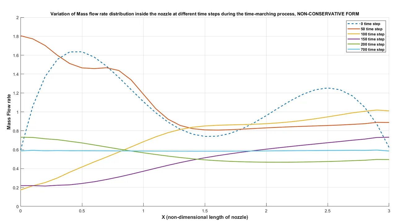
From the above plot, we can see that mass flow rate variation throughout the nozzle is too high for time step 0 & 50, its because just the fluid entered and there will be a lot of variation in the flow at initial time stages but going forward at time step 150 & 200 the variations in mass flow are gradually reduced throughout the nozzle and by 700th-time step, it almost reached the steady value.
Conservative form:
function[frho,ft,fv,pressu,mach,local_massflow,totalmf,throat_mach] = cons2(nt,n,x,dx,dt,rho,t,v,a,throat,gamma)
    %intialization with zero
    throat_v=zeros(1,nt);
    throat_t=zeros(1,nt);
    throat_rho=zeros(1,nt);
    throat_p=zeros(1,nt);
    throat_mach=zeros(1,nt);
    local_massflow=zeros(nt,n);
    start_massflow = rho.*v.*a;
    %defining initial conditions
    u1=rho.*a;
    u2=rho.*a.*v;
    u3= rho.*a.*((t/(gamma-1)+((gamma/2)*(v.^2))));
    %outer time loop
    for k=1:nt
       u1_old=u1;
       u2_old =u2;
       u3_old=u3;
       %flux terms
       f1=u2;
       f2=u2.^2./u1+((gamma-1)/gamma).*(u3-(gamma/2)*u2.^2./u1);
       f3=gamma.*u2.*u3./u1-0.5*gamma*(gamma-1).*u2.^3./u1.^2;
       %predictor step
        for i=2:(n-1) %for inner loop
            j2= (1/gamma)*rho(i)*t(i)*(a(i+1)-a(i))/dx; %%ERROR : (a(i+1)-a(i))/dx
            du1dt_p(i)=-((f1(i+1)-f1(i))/dx);
            du2dt_p(i)=-((f2(i+1)-f2(i))/dx)+j2;
            du3dt_p(i)=-((f3(i+1)-f3(i))/dx);
            %updating solution vector
            u1(i)= (du1dt_p(i)*dt)+u1_old(i);
            u2(i)= (du2dt_p(i)*dt)+u2_old(i);
            u3(i)= (du3dt_p(i)*dt)+u3_old(i);
        end
        %Update for corrector step
        f1=u2;
        f2=u2.^2./u1+((gamma-1)/gamma).*(u3-(gamma/2)*u2.^2./u1);
        f3=gamma.*u2.*u3./u1-0.5*gamma*(gamma-1).*u2.^3./u1.^2;
        rho=u1./a;
        t=(gamma-1).*(u3./u1-(gamma/2).*(u2./u1).^2);
        %corrector step
        for j=2:(n-1) %for inner loop
            %j2= ((gamma-1)/gamma)*(u3 - (gamma/2)*((u2.^2)./(u1.^2)))*((log(a(j))-log(a(j-1)))/dx);
            j2= (1/gamma)*rho(j)*t(j)*(a(j)-a(j-1))/dx; %%ERROR : (a(i+1)-a(i))/dx
            du1dt_c(j)=-((f1(j)-f1(j-1))/dx);
            du2dt_c(j)=-((f2(j)-f2(j-1))/dx)+j2;
            du3dt_c(j)=-((f3(j)-f3(j-1))/dx);
        end
        %compute average time derivative
        du1dt_avg = 0.5*(du1dt_p+du1dt_c);
        du2dt_avg = 0.5*(du2dt_p+du2dt_c);
        du3dt_avg = 0.5*(du3dt_p+du3dt_c);
        %final solution update
        for h=2:n-1
            u1(h)=dt*du1dt_avg(h)+u1_old(h);
            u2(h)=dt*du2dt_avg(h)+u2_old(h);
            u3(h)=dt*du3dt_avg(h)+u3_old(h);
        end
        %applying boundary conditions
        %inlet
        u1(1)=a(1);
        u2(1)=2*u2(2)-u2(3);
        v(1)= u2(1)/u1(1);
        u3(1)=u1(1)*((t(1)/(gamma-1))+(gamma/2)*(v(1)^2));
        %outlet
        u1(n)=2*u1(n-1)-u1(n-2);
        u2(n)=2*u2(n-1)-u2(n-2);
        u3(n)=2*u3(n-1)-u3(n-2);
        %calculating primitive variables
        rho=u1./a;
        v=u2./u1;
        t=(gamma-1)*((u3./u1)-((gamma/2)*v.^2));
        %local pressure calculation
        p=rho.*t;
        %local mach number calculation
        mach = v./((t).^0.5);
        throat_rho(k)=rho(throat);
        throat_v(k)=v(throat);
        throat_t(k)=t(throat);
        throat_p(k)=p(throat);
        throat_mach(k)=mach(throat);
        %mass flow calculations
        %overall mass flow through nozzle
        inflow = rho(1)*v(1)*a(1);
        outflow = rho(n)*v(n)*a(n);
        totalmf(k) = outflow-inflow;
        local_massflow(k,:) = rho.*v.*a;
    end
    %final solution
    frho=rho;
    ft=t;
    fv=v;
    pressu=p;
    %plots
    figure(3)
    subplot(5,1,1)
    plot(throat_rho,'linewidth',1.5)
    grid on
    xlabel('no.of timestep')
    ylabel('Rho''')
    legend('Density'' at throat')
    title('nt vs density')
    subplot(5,1,2)
    plot(throat_t,'linewidth',1.5)
    xlabel('no.of timestep')
    ylabel('Temp.''')
    legend('Temperature'' at throat')
    title('nt vs temp')
    grid on
    subplot(5,1,3)
    plot(throat_p,'linewidth',1.5)
    xlabel('no.of timestep')
    ylabel('P''')
    legend('Pressure'' at throat')
    title('nt vs pressure')
    grid on
    subplot(5,1,4)
    plot(throat_mach,'linewidth',1.5)
    xlabel('no.of timestep')
    ylabel('Mach')
    legend('Mach at throat')
    title('nt vs mach number')
    grid on
    subplot(5,1,5)
    plot(totalmf,'linewidth',1.5)
    xlabel('no.of timestep')
    ylabel('M.F''')
    legend('Total Mass Flow at throat')
    title('nt vs total mass flow')
    grid on
    sgtitle('Time-wise variation of the primitive variables at throat')

    figure(4)
    hold on
    plot(x,start_massflow,'--','linewidth',1.75)
    plot(x,local_massflow(100,:),'linewidth',1.75)
    plot(x,local_massflow(200,:),'linewidth',1.75)
    plot(x,local_massflow(300,:),'linewidth',1.75)
    plot(x,local_massflow(400,:),'linewidth',1.75)
    plot(x,local_massflow(1400,:),'linewidth',1.75)
    ylabel('Mass Flow rate')
    xlabel('X (non-dimensional length of nozzle)')
    legend('0 time step','100 time step','200 time step','300 time step','400 time step','1400 time step')
    grid on
    title({['Variation of Mass flow rate distribution inside the nozzle at different time steps during the time-marching process, CONSERVATIVE FORM'],['n=61, nt=2800']})
    hold off
end
Results form the 3rd part(conservative form):
Figure(1):
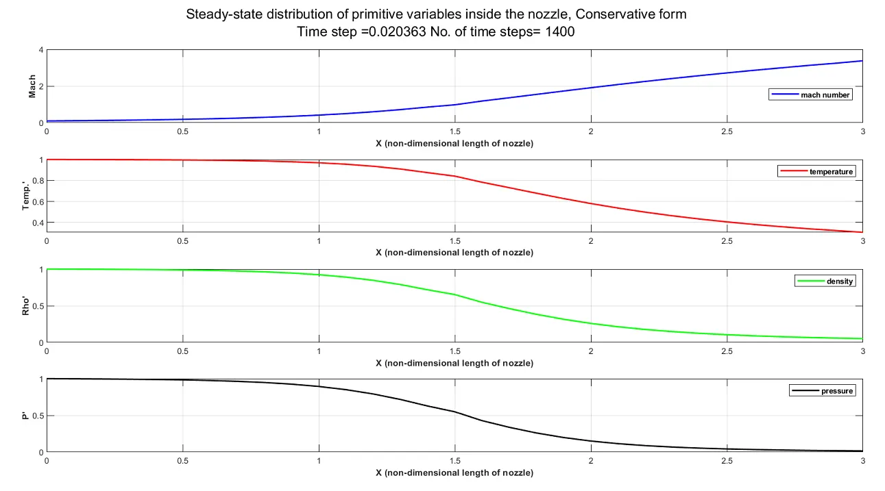
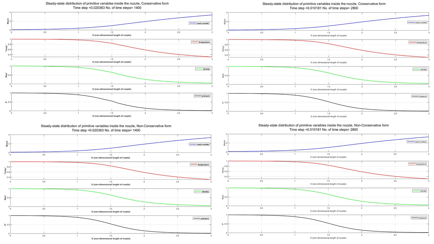
From the variation of pressure, temperature, velocity, and density throughout the nozzle for both conservative and non-conservative forms all the parameters are the same. As expected in the initial case Mach number at throat for both cases is 1. So while comparing these four parameters both the cases yield the same result.
Figure(2):
Figure(3):
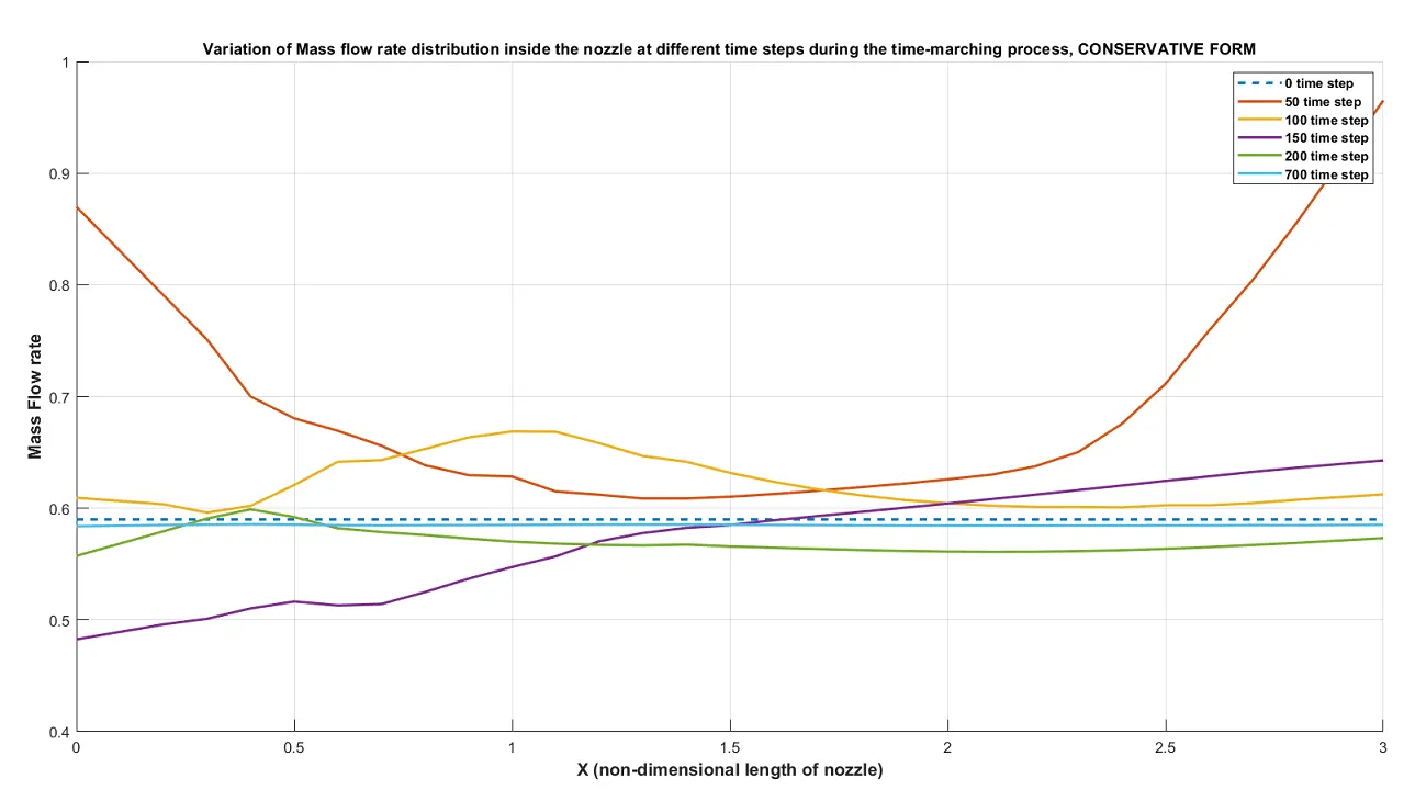
From the above plot, we can see that mass flow rate variation throughout the nozzle is too high for time step 50 its because just the fluid entered and there will be a lot of variation in the flow at initial time stages but going forward at time step 150 and 200 the variations in mass flow are gradually reduced throughout the nozzle and by 700th-time-step, it almost reached the steady value. One thing that can be seen as a difference in the conservative and non-conservative form here is the maximum value in mass flow.
Thus we can conclude for practical purposes both forms of governing equations will give the same results when the flow problem studied in both cases is isentropic, subsonic-supersonic flow through a nozzle. In those cases, the non-conservative and conservative form won't make much difference. But there will be a considerable change in both governing equations if we try to capture the shock wave capturing.
Comparison of Normalized mass flow rate distributions of both forms
Figure(4):
Grid-Independent test:
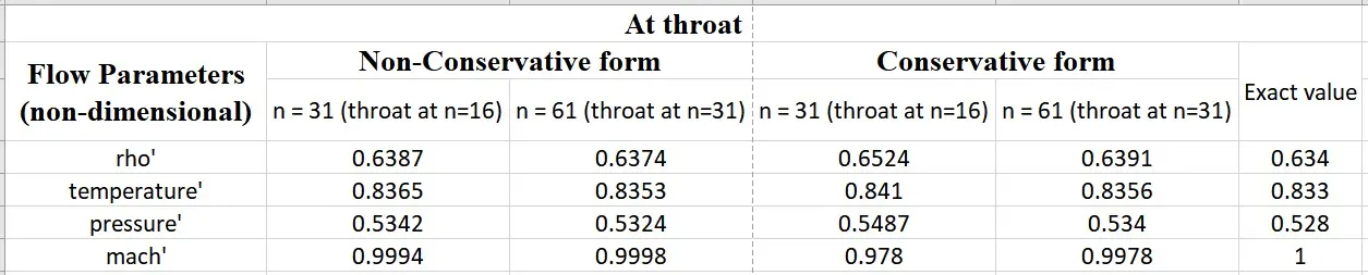
In order to conduct a grid dependency test, here two situations are considered one with 31 grid points and other with 61 grid points. Values here shown are from the grid where the throat area lies. From the below table it can be seen that the increase in grid point will increase the accuracy but the run of the simulation also drastically increase with the increase in the number of grid points. It means that faster result is less accurate.
The results of the grid dependency test can be compared in the below graphs:
Comparison of Figure(1):
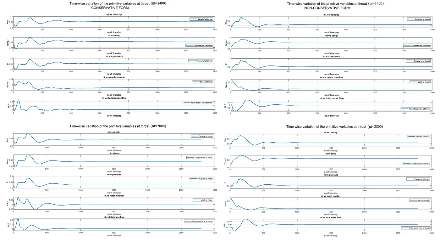
Comparison of Figure(2):
Comparison of Figure(3):
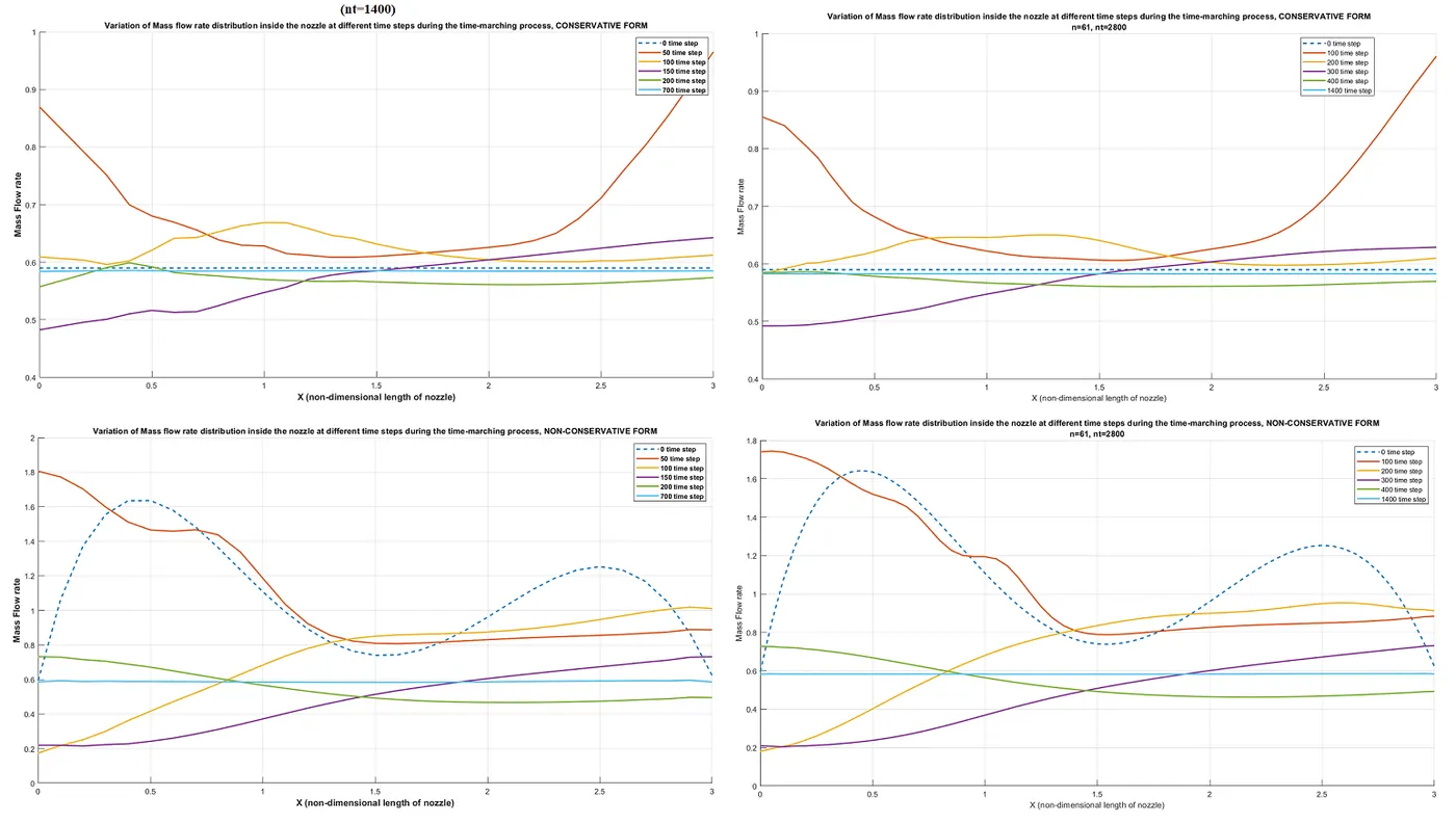
Comparison of Figure(4):
CONCLUSION:
- After comparing both the methods it has been seen that there are a lot more fluctuations in nonconservative one when compared to the conservative one.
- After comparing both the forms in terms of execution time the non-conservative form is faster when compared to a conservative form. The main reason is the conservative part has more mathematical calculations.
- Non-Conservative form converges more quickly after 300 iterations, the solution starts converging whereas the conservative part starts converging after 400 iterations.
- Complexity in solving the conservative form is more when compared to non-conservative since the conservative part has more mathematical calculation when compared to nonconservative form