Week 9 - FVM Literature Review

Finite Volume Method (FVM) is a numerical method used to solve partial differential equations by discretizing the domain into small control volumes or cells. In FVM, the governing equations are integrated over each control volume, which leads to a set of algebraic equations that can be solved using numerical methods.

The major differences between Finite Difference Method (FDM) and FVM are as follows:

1. In FDM, the domain is discretized into a grid of points, whereas in FVM, the domain is discretized into control volumes.
2. In FDM, the values of the solution are stored at the grid points, whereas in FVM, the values are stored at the control volume centers.
3. In FDM, the derivatives are approximated using the values of the solution at neighboring grid points, whereas in FVM, the derivatives are approximated by integrating the fluxes across the faces of the control volumes.

Interpolation schemes and flux limiters are needed in FVM to ensure accurate and stable solutions. Interpolation schemes are used to compute the values of the solution at the faces of the control volumes, which are required to compute the fluxes. Flux limiters are used to limit the magnitude of the numerical fluxes to prevent spurious oscillations and ensure stability of the solution.

As an example, let's consider the 1D linear heat conduction equation:

$$ \frac{\partial T}{\partial t} = \alpha \frac{\partial^2 T}{\partial x^2} $$

where $T$ is the temperature, $\alpha$ is the thermal diffusivity, $t$ is time, and $x$ is the spatial coordinate.

To apply FVM to this equation, we first discretize the domain into control volumes with centers at $x_i$ and faces at $x_{i-1/2}$ and $x_{i+1/2}$, as shown in the figure below:

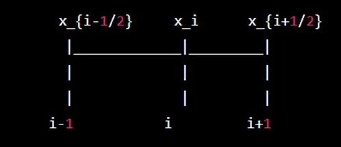
The heat conduction equation is then integrated over the control volume $i$:

$$ \int_{x_{i-1/2}}^{x_{i+1/2}} \frac{\partial T}{\partial t} dx = \alpha \int_{x_{i-1/2}}^{x_{i+1/2}} \frac{\partial^2 T}{\partial x^2} dx $$

Using the divergence theorem, we can express the second integral as a surface integral of the flux:

$$ \alpha \int_{x_{i-1/2}}^{x_{i+1/2}} \frac{\partial^2 T}{\partial x^2} dx = \alpha [ \frac{\partial T}{\partial x} ]{x{i-1/2}}^{x_{i+1/2}} $$

Assuming a constant thermal diffusivity, we can simplify the equation as:

$$ \frac{T_i^{n+1} - T_i^n}{\Delta t} = \frac{\alpha}{\Delta x^2} (T_{i-1}^n - 2 T_i^n + T_{i+1}^n) $$

where $T_i^n$ is the temperature at the center of control volume $i$ at time level $n$, and $\Delta t$ and $\Delta x$ are the time and spatial step sizes, respectively.

To compute the fluxes at the faces of the control volumes, we need to interpolate the values of the solution from the control volume centers to the faces. One common interpolation scheme used in FVM is the piecewise linear interpolation, which assumes that the solution is linear within each control volume. The value of the solution at the face $x_{i+1/2}$ is then computed as:

$$T_{i+1/2} = \frac{T_{i+1}+T_i}{2} + \frac{\Delta x}{2} \frac{\partial T}{\partial x} $$

Similarly, the value of the solution at the face $x_{i-1/2}$ is computed as:

$$T_{i-1/2} = \frac{T_i+T_{i-1}}{2} - \frac{\Delta x}{2} \frac{\partial T}{\partial x} $$

Once we have the values of the solution at the faces, we can compute the numerical fluxes using a discretization scheme. One common discretization scheme used in FVM is the central difference scheme, which approximates the derivative as:

$$\frac{\partial T}{\partial x} \approx \frac{T_{i+1/2} - T_{i-1/2}}{\Delta x} $$

The numerical flux at the face $x_{i+1/2}$ is then computed as:

$$F_{i+1/2} = -\alpha \frac{T_{i+1/2} - T_{i-1/2}}{\Delta x} $$

Similarly, the numerical flux at the face $x_{i-1/2}$ is computed as:

$$F_{i-1/2} = -\alpha \frac{T_{i-1/2} - T_{i-3/2}}{\Delta x} $$

Finally, we apply a flux limiter to limit the magnitude of the numerical fluxes to prevent spurious oscillations and ensure stability of the solution. One common flux limiter used in FVM is the minmod limiter, which selects the minimum of the upwind and downwind slopes:

$$\phi(r) = \begin{cases} 0 & r \leq 0 \ \min(1, r) & 0 < r < 1 \ 1 & r \geq 1 \end{cases} $$

where $r$ is the ratio of the upwind and downwind slopes:

$$r = \frac{T_i - T_{i-1}}{T_{i+1} - T_i} $$

The numerical flux at the face $x_{i+1/2}$ is then modified as:

$$\tilde{F}{i+1/2} = F{i+1/2} \phi(r) $$

Similarly, the numerical flux at the face $x_{i-1/2}$ is modified as:

$$\tilde{F}{i-1/2} = F{i-1/2} \phi(-r) $$

Overall, the Finite Volume Method is a powerful numerical method for solving partial differential equations. By discretizing the domain into control volumes and integrating the governing equations over each control volume, we can obtain a set of algebraic equations that can be solved using numerical methods. However, to ensure accurate and stable solutions, we need to use interpolation schemes and flux limiters to compute the values of the solution at the faces of the control volumes and limit the magnitude of the numerical fluxes.