Week 9 - FVM Literature Review
What is Finite Volume Method(FVM),
Computational fluid dynamics (CFD) is a branch of fluid mechanics that uses numerical analysis and data structures to analyze and solve problems that involve fluid flows.
Methodology For CFD Analysis:
The Geometry Is designed using the CAD Software.
The volume occupied by the fluid is divided into no of cells called as mesh.
The physiscal model is defined ie the equations of fluid motion.
Boundary conditions are defined. This involves specifying the fluid behaviour and properties at all bounding surfaces of the fluid domain. For transient problems, the initial conditions are also defined.
The simulation is started and the equations are solved iteratively as a steady-state or transient.
Finally a postprocessor is used for the analysis and visualization of the resulting solution.
Discretization methods
Some of the discretization methods being used are:
Finite volume method
In the finite volume method, the governing partial differential equations (typically the Navier-Stokes equations, the mass and energy conservation equations, and the turbulence equations) are recast in a conservative form, and then solved over discrete control volumes. This discretization guarantees the conservation of fluxes through a particular control volume. The finite volume equation yields governing equations in the form
`del/(delt)intintintQdV+intintFdA=0`
Finite element method
The finite element method (FEM) is used in structural analysis of solids, but is also applicable to fluids. However, the FEM formulation requires special care to ensure a conservative solution. The FEM formulation has been adapted for use with fluid dynamics governing equations. Although FEM must be carefully formulated to be conservative, it is much more stable than the finite volume approach. However, FEM can require more memory and has slower solution times than the FVM.
Finite difference method
The finite difference method (FDM) has historical importance and is simple to program. It is currently only used in few specialized codes, which handle complex geometry with high accuracy and efficiency by using embedded boundaries or overlapping grids (with the solution interpolated across each grid).
Finite Volume method
The finite volume method (FVM) is a method for representing and evaluating partial differential equations in the form of algebraic equations.
In the finite volume method, volume integrals in a partial differential equation that contain a divergence term are converted to surface integrals, using the divergence theorem. These terms are then evaluated as fluxes at the surfaces of each finite volume. Because the flux entering a given volume is identical to that leaving the adjacent volume, these methods are conservative. Another advantage of the finite volume method is that it is easily formulated to allow for unstructured meshes. The method is used in many computational fluid dynamics packages. "Finite volume" refers to the small volume surrounding each node point on a mesh.
write down the major differences between FDM & FVM.
In finite difference method the dependent variable values are stored at the nodes only. Infinite element method, the dependent values are stored at the element nodes. But in finite volume method, the dependent values are stored in the centre of the finite volume.
Finite difference method cannot be used in the complex geometries where the grid is not alligned in x, y and Z directions.
Instead of writing the equations in a point, we write it for a volume.
Finite Volume Method is the numerical method that solves a governing equation in its integral form, that mean the variable properties are conserved over a volume rather than a point as in case of Finite Difference Method.
Finite Volume method(FVM) uses integral form of governing whereas the Finite Difference method(FDM) uses differential form of the governing equations. The discretised equation in the FVM has a clear physical interpretation while in the FDM is not that clearly interpreted.
Also, describe the need for interpolation schemes and flux limiters in FVM. You can use the 1D linear heat conduction equation as an example.
Types of Interpolation schemes:
1) Upwind Interpolation scheme
2) Linear Interpolation scheme
3) Quadratic Upwind Interpolation scheme
4) Hybrid scheme
5) Total Variation Diminishing (TVD)scheme
Consider the 1D Steady State Heat Conduction equation, where F.V.M. is applied,
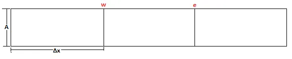
Consider the 1-D steady state equation with heat generation
`del/(delx)(alpha(delT)/(delx))+S=0`
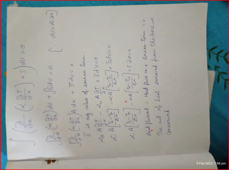
The Finite Difference Method, having non-conservative form of equations, does not involve integration on a particular control volume, so Gauss Divergence Theorem cannot be used, so the F.D.M. will not result in conservation on cell by cell(elemental) basis, whereas this is satisfied by the Finite Volume Method.
The final solution of a simulation will be same by the Finite Volume or by the Finite Difference Method, however the path to the solution is different. The goes thru the sequence of conservation equations for Finite Volume Method, whilst via Finite Difference Method, it may not go conserved.
Need for Interpolation schemes :
We need interpolation schemes to find the value of properties at the boundaries of the control volumes.
If we want to find out the value of thermal conductivity at a boundary of a control volume and if it a function of temperature we will have to interpolate the values of the temperature from the neighbouring nodes to find the temperature at the boundary and that only we will be able to find the value of thermal conductivity at that boundary.
Need for Flux Limiter:
While calculations for the interpolations there might be sudden jump in the values of fluxes due to shocks in the system this can create errors and may even blow up our solutions so to limit the values of fluxes we need to provide flux limiters.
Most of us might have seen the behaviour of numerical schemes in order to capture shocks and discontinuity that arises in hyperbolic equations. Physically, these equations model the convective fluid flow. It has been observed that low-order schemes are usually stable but quite dissipative in nature around the points of discontinuity/shocks. On the other hand higher-order numerical schemes are unstable in nature and show oscillations in the vicinity of discontinuity. One can have a better understanding of such behaviour by analysing the modified equation of these schemes.
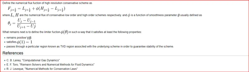
Now as said above one can not have high order accuracy without oscillations. The objective is to have highly accurate and stable oscillation free schemes. This kind of schemes are known as high resolution schemes. In 1984 Harten proposed the constuction and gave TVD criteria for such scheme. Here we talk only about using flux limiters function to construct high resolution schemes. The idea is to tune the numerical flux of high order and low order scheme using the flux limiter function in such a way that the resulting scheme gives a high order accuracy in the smooth region of flow and sticks with first order of accuracy in the vicinity of socks/discontinuities as follows: