Week 9 - FVM Literature Review

AIM

FVM literature review

Finite Volume Method

A finite volume method (FVM) discretization is based upon an integral form of the PDE to be solved (e.g. conservation of mass, momentum, or energy). The PDE is written in a form which can be solved for a given finite volume (or cell). The computational domain is discretized into finite volumes and then for every volume the governing equations are solved.

Major Differences between FVM And FDM

• A finite difference method (FDM) discretization is based upon the differential form of the PDE to be solved.
• Each derivative is replaced with an approximate difference formula (that can generally be derived from a Taylor series expansion). The computational domain is usually divided into hexahedral cells (the grid), and the solution will be obtained at each nodal point.
• The discretization results in a system of equation of the variable at nodal points, and once a solution is found, then we have a discrete representation of the solution.
• A finite volume method (FVM) discretization is based upon an integral form of the PDE to be solved (e.g. conservation of mass, momentum, or energy).
• The PDE is written in a form which can be solved for a given finite volume (or cell).
• The computational domain is discretized into finite volumes and then for every volume the governing equations are solved. The resulting system of equations usually involves fluxes of the conserved variable, and thus the calculation of fluxes is very important in FVM.
• The basic advantage of this method over FDM is it does not require the use of structured grids, and the effort to convert the given mesh in to structured numerical grid internally is completely avoided.
• As with FDM, the resulting approximate solution is a discrete, but the variables are typically placed at cell centers rather than at nodal points. This is not always true, as there are also face-centered finite volume methods. In any case, the values of field variables at non-storage locations (e.g. vertices) are obtained using interpolation.
• A finite element method (FEM) discretization is based upon a piecewise representation of the solution in terms of specified basis functions. The computational domain is divided up into smaller domains (finite elements) and the solution in each element is constructed from the basis functions.
  
• FVM and FDM provide discrete solutions, while FEM provides a continuous (up to a point) solution. FVM and FDM are generally considered easier to program than FEM, but opinions vary on this point. FVM are generally expected to provide better conservation properties, but opinions vary on this point also. If you are trying to decide which method to use, then the best path is probably found by consulting the literature in the specific problem area.

Finite volume method for onedimensional steady state diffusion

Governing equation

`d/dx(Γ(dΦ /dx) )+S=0`

Where Γ is the diffusion coefficient and S is the source term. Boundary values of φ at points A and B are prescribed.

Control volume

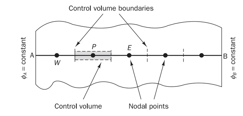
Step 1 -Grid generation

The first step in the finite volume method is to divide the domain into discrete control volumes. Let us place a number of nodal points in the space between A and B. The boundaries (or faces) of control volumes are positioned mid-way between adjacent nodes. Thus each node is surrounded by a control volume or cell. It is common practice to set up control volumes near the edge of the domain in such a way that the physical boundaries coincide with the control volume boundaries

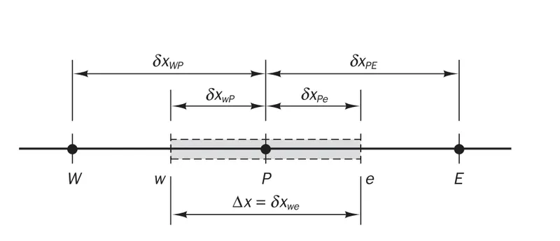
• A general nodal point is identified by P and its neighbours in a onedimensional geometry, the nodes to the west and east, are identified by W and E respectively.
• The west side face of the control volume is referred to by w and the east side control volume face by e. The distances between the nodes W and P, and between nodes P and E, are identified by δxWP and δxPE respectively.
• Similarly distances between face w and point P and between P and face e are denoted by δxwP and δxPe respectively. Figure 4.2 shows that the control volume width is ∆x = δxwe.

Step 2-Discretisation

• The key step of the finite volume method is the integration of the governing equation (or equations) over a control volume to yield a discretised equation at its nodal point P.
• For the control volume defined above this gives

• Here A is the cross-sectional area of the control volume face, ∆V is the volume and D is the average value of source S over the control volume.
• It is a very attractive feature of the finite volume method that the discretised equation has a clear physical interpretation. Equation states that the diffusive flux of φ leaving the east face minus the diffusive flux of φ entering the west face is equal to the generation of φ, i.e. it constitutes a balance equation for φ over the control volume.
• In order to derive useful forms of the discretised equations, the interface diffusion coefficient Γ and the gradient dφ/dx at east (e) and west (w) are required.
• The values of the property φ and the diffusion coefficient are defined and evaluated at nodal points. To calculate gradients (and hence fluxes) at the control volume faces an approximate distribution of properties between nodal points is used.
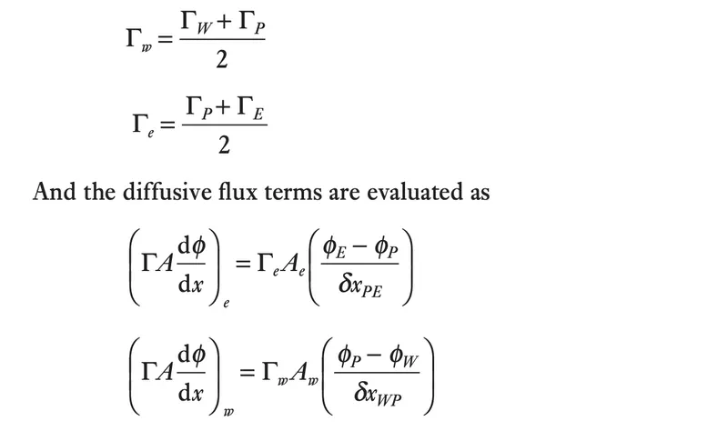
• Linear approximations seem to be the obvious and simplest way of calculating interface values and the gradients. This practice is called central differencing
• .And the diffusive flux terms are evaluated as

• In practical situations, the source term S may be a function of the dependent variable. In such cases the finite volume method approximates the source term by means of a linear form:

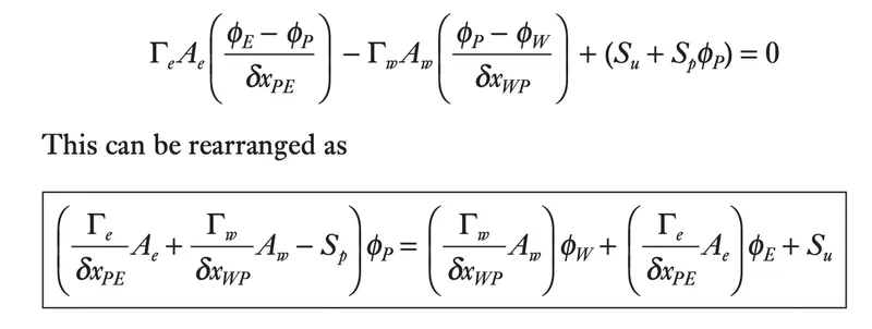
Substituting the above two equations in this equation gives

Step 3-Solution of equations

Discretised equations of the form must be set up at each of the nodal points in order to solve a problem. For control volumes that are adjacent to the domain boundaries the general discretised equation is modified to incorporate boundary conditions. The resulting system of linear algebraic equations is then solved to obtain the distribution of the property φ at nodal points

Need for interpolation schemes:

To calculate the Tw and Te, Temperature at the west and east faces, we have the value at the Tp,Te,andTw by interpolating the values, we can get the temperature at the east and west faces. By using them we can calculate the thermal diffusivity of the faces are αe and αw .There are different ways of Interpolation. Some of the ways are given by

• Upwind interpolation scheme.
• Linear Interpolation scheme.
• Quadratic Interpolation scheme.
• Hybrid Interpolation Scheme.

Flux limiters

In solving the convective flow fields, it is observed that the discontinuity or shocks in results. For the High order, it is observed that the Oscillation is more and the solution became unstable due to this reason.

To obtain the highly accurate and oscillation free results we need to use the flux limiter function. The function provides the smooth region over the flow and maintains the first-order accuracy. Flux limiters are mainly used to get the total variation diminishing [TVD].

Their simple forms for 1D Equation are given by

`(du)/dt+1/(Δx)[F(u+1/2)−F(u-1/2)]=0`

Reference

• An Introduction to Computational Fluid Dynamics THE FINITE VOLUME METHOD - H K Versteeg and W Malalaseker

• Wikipedia