Week 9 - FVM Literature Review

Finite Volume Method
This method involves descretizing the domain into finite number of control volumes. Then solving the governing differential equations for each Control Volume to solve the problem for the entire domain. One of the major difference between Finite Difference method and Finite volume method is the way the domain is discretized. Finite Difference method takes into account information at points in space but in Finite volume method the information is intrinsic to a stencil control volume which is obtained by discretizing the whole domain or space into small control Volumes.

To understand it better, lets consider a case of fluid of density rho and coefficient of diffusion `Gamma` flowing through a one dimensional domain of length L and cross-sectional area A. We will assume that fluid velocity field and scalar quantities such as density and coefficient of diffusion remain constant with respect to time. We will assume that Temperature of fluid at the inlet and at the outlet will be constant through out the time it reaches steady state. We are going to consider a case of temperature distribution in a fluid due to conduction and diffusion at a steady state.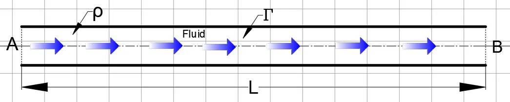

So according to Reynold's Transport Theorem
`int_V (del(rho*phi))/(delt).dv+int_S (rhophi*u)*hat n ds=int_S (Gamma .grad(phi))*hat n ds+int_V S_phi.dv`
Where `phi`is any scalar property that is non-uniformly distributed in space which is affected by both velocity of fluid (conduction) and diffusion of that scalar property (diffusion). This scalar property can have direct relation with velocity field or can be bereft of it. Here the scalar property phi is temperature and this scalar property does not affect the vector field.
Now in this case, since steady state is required the transient term changes to zero and it is assumed that the source is absent through out the domain and hence the source term is also cancelled. So the equation becomes:-
`int_S (rhophi*u)*hat n ds=int_S (Gamma .grad(phi))*hat n ds`
Now applying divergence theorem to the above integral equation, we get
`int_v grad*(rhophiu)*dv=int_v grad*(Gamma .grad(phi)) dv`
Now imagine the whole domain descritized into control volumes in the following way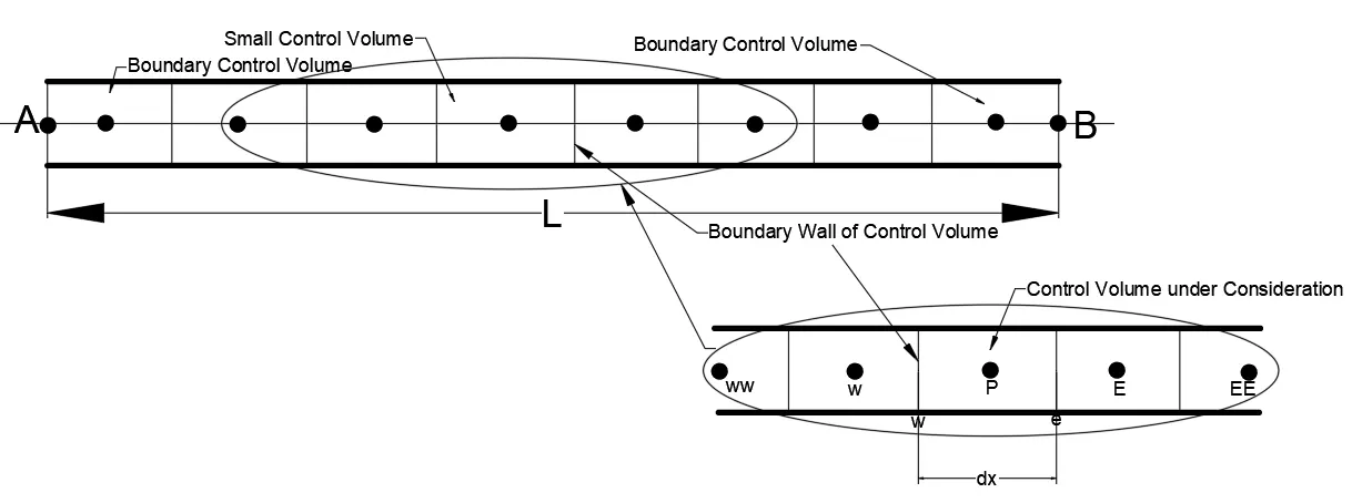

The above domain, as displayed, is distributed into a series of control volumes. The control volumes at the domain boundary are displayed. In the ellipse, a sample control volume is taken into consideration. The control volume with central node P is the C.V. under consideration. The control Volumes with node W and E are the nodes of Control Volume abutting the C.V. under consideration.And WW and EE are respectively nodes of C.V. further away from C.V. with node P as denoted by the above figure. It is assumed that the flow is considered positive when velocity of fluid is from W to E and negative otherwise.The West and East boundary wall C.V. with node P are denoted by w and e.
Before going into descritization, lets establish a function to give out exact solution of the above problem:-
`(phi-phi_0)/(phi_L-phi_0)=(exp((rhoux)/Gamma)-1)/(exp((rhouL)/Gamma)-1)`
This equation is converted into a function:-

function [phi]=Exact_diffusion_Convection_Solver(rho,u,T,phi0,phiL,x)
L=abs(x(end)-x(1));
K=rho*u/T;
phi=phi0+((phiL-phi0)/(exp(K*L)-1))*(exp(K*x)-1);
end

The governing integral equation is applied across a elemental control volume which is denoted by central node P. The length of the control volume is dx and cross-sectional area is A.
`int_v (del(rhophiu))/(delx)*A.dx=int_v (del(Gamma .(delphi)/(delx)))/(delx) A.dx`
Now simplifying above equation and applying numerical formula for derivatives, we get
`(rhophiu)_e-(rhophiu)_w=(Gamma .(delphi)/(delx))_e-(Gamma .(delphi)/(delx))_w`
A is cancelled in the above equation since A is constant at every point in the domain.
Now let `F=rhou`
`D=Gamma/dx`
So further simplifying we get
`F_ephi_e-F_wphi_w=D_e(phi_E-phi_P)-D_w(phi_P-phi_W)`
....this is governing numerical equation across a control volume. Here central differencing is applied at derivative in diffusion term.
Now when a computer programming is employed to solve these equations. It is assumed that the information is known at all centroid of these control volumes and at 2 boundary nodes of domain. The value of phi is not known at the boundary walls of the control volume. So `phi_e and phi_w`are not known.
Now to calculate phi_w and phi_e, different interpolation schemes are employed which use values at centre nodes of neighbouring control volumes to calculate values of phi at boundary walls e and w of control volume with centre node P.
Now there are various interpolation schemes that are employed which will be explored one by one. First it is important to set case study of the problem set for these schemes.
First it is to be understood that phi variable is used as a scalar field variable to study the schemes. But we just have to consider phi as temperature to make the problem for convection and diffusion of fluid.
Let temperature at the inlet=373 K=`phi_A`
temperature at the outlet = 272 K=`phi_B`
Length of the domain=L=1m
Lets consider a imaginary fluid for the sake of convenience
Density of fluid=1 kg/`m^3`
Thermal diffusivity of water=0.1 W/mK
Fluid velocity will not be affected by scalar field variable phi or T as in this case. Three values of velocity will be taken to study the case
1)0.1m/s
2)0.5 m/s
3)2.5 m/s
Occasionally velocity examples may be added to explain the interpolation method in a better way. Understand this that a code will be drafted in matlab to solve the case.
The number of Control volumes=n
This number n will also be a variable. to show effect to effect of course or fine mesh on stability or accuracy of solution for a particular interpolation method employed.
The number of node points=nx=n+2
The number of node points is n+2 because all the centre nodes of the control volume is counted along with the nodes at the border at A and B. Also remember that though centrol nodes are at a distance of dx from central nodes of neighbour control volumes, the node at A is at a distance of dx/2 from node 1 and node at B is at a distance dx/2 from the central node of control volume at the end. Moreover another point to be noted is that if a node number is z, then its position number is z+1 in the code.
Lets one by one enumerate interpolation methods , apply them in the form of a code and then understand its advantages and disadvantages.

1) Central Differencing Scheme

So in this scheme, it is considered that the `phi_e and phi_w` are
`phi_e=(phi_P+phi_E)/2`
`phi_w=(phi_P+phi_W)/2`
Now it must be puzzling that how is this scheme central differencing. Now if we go back to the derivation of original equation, we will find that
`(del(rhophiu))/(delx)|_P=(F_ephi_e-F_wphi_w)/dx`
This `(del(rhophiu))/(delx)`is basically derivative at P
Now when substitution of interpolation is done, citing that Fe=Fw, it will be found that
`(del(rhophiu))/(delx)|_P=(F_e(phi_P+phi_E)/2-F_w(phi_P+phi_W)/2)/dx=F(phi_E-phi_W)/(2*dx)`
Which is what we have learnt is the formula of first order derivative using central differencing. Thats why the scheme is called central differencing because the interpolation scheme ultimately leads to the central differencing formula. And this makes the scheme of 2nd order approximation.
So when the the interpolation scheme is substituted in the numerical governing differential equation, following form of equation is obtained.
`F_e((phi_P+phi_E)/2)-F_w((phi_P+phi_W)/2)=D_e(phi_E-phi_P)-D_w(phi_P-phi_W)`
And after rearranging it becomes of this form
`a_Pphi_P=a_Wphi_W+a_Ephi_E`
where
`a_W=D_w+F_w/2`
`a_E=D_e-F_e/2`
`a_P=a_W+a_E+F_e-F_w`
Now it is understood that solving governing differential equation is difficult but iterative methods can be employed to solve algebraic equation. This equation is used for every node except border nodes to solve the equation.
The case for border node is a little different. It has to be treated as a special case. This because there is no central node of the control volume to the west of 1st control volume and no central node of the control volume to the east of control volume at the end.
So for node one the governing numerical differential equation becomes
`F_e((phi_P+phi_E)/2)-F_AphiA=D_e(phi_E-phi_P)-D_A(phi_P-phi_A)`
Now F_A=Fw....the normal formula
but imagining a mirror node `phi_W`beyond phi at A, then it can be said that
`phi_P-phi_A=phi_A-phi_W`
this further makes the equation
`phi_P-phi_W=2(phi_P-phiA)`
now this makes
`D_A=2*D_W=2D`
So the equation finally becomes
`a_Pphi_P=a_Ephi_E+(D_A+F_A)phiA`
where
`a_E=D_e-F_e/2`
`a_P=a_E+D_A+F_A+Fe-FA`
Similarly for node 5, the equation becomes
`F_BphiB-F_w((phi_P+phi_W)/2)=D_B(phi_B-phi_P)-D_w(phi_P-phi_W)`
`D_B=2*D_e=2D`and `F_B=F_e`
so finally the equation becomes
`a_Pphi_P=a_Wphi_W+(D_B-F_B)phiB`
where
`a_W=D_w+F_w/2`
`a_P=a_W+F_B-F_w`
Now to encompass all the nodes including the ones at the border into a single equation, we get
`a_Pphi_P=a_Wphi_W+a_Ephi_E+Su`
where
`a_P=a_W+a_E+Sp+F_e-F_w`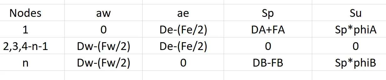

Now this equation is transformed into a code and solved using Gauss seidel iterative solver in matlab as follows

clear all
close all
clc
%Input

n=5;
L=1;%in meter
rho=1;%kg/m^3
T=0.1;
u=0.1;%m/s

%Derived Values

F=rho*u;
dx=L/n;
D=T/dx;
nx=n+2;% Position number

%Domain

x(1)=0;
x(2:nx-1)=(dx/2):dx:(L-(dx/2));
x(nx)=L;

%Initial Output

phiA=373;
phiB=273;
phi=zeros(1,nx);
phi(1)=phiA;
phi(nx)=phiB;

%Iteration Settings

tol=1e-5;
error=9e9;

%Solver
while(error>tol)
phiold=phi;
for i=2:nx-1
if i==2
   aw=0;
   Aw=0;
   Sp=2*D+F;
   Su=Sp*phiA;
else
   aw=D+(F/2);
   Aw=aw*phi(1,i-1);
end
if i==(nx-1)
   ae=0;
   Ae=0;
   Sp=2*D-F;
   Su=Sp*phiB;
else
   ae=D-(F/2);
   Ae=ae*phiold(1,i+1);
end
if i~=2
  if i~=nx-1
Sp=0;
Su=0;
  end
end
ap=aw+ae+Sp;
phi(1,i)=(Ae+Aw+Su)/ap;  
end
error=max(abs(phi-phiold));
end
[phi_exact]=Exact_diffusion_Convection_Solver(rho,u,T,phiA,phiB,x)
plot(x,phi)
hold on
plot(x,phi_exact,'--')
xlabel('x')
ylabel('Temperature')
title('Temperature Distribution')
legend('Numerical Solution','Exact Solution')

when n=5

1) u=0.1m/s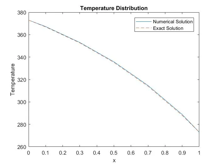

2) u=0.5m/s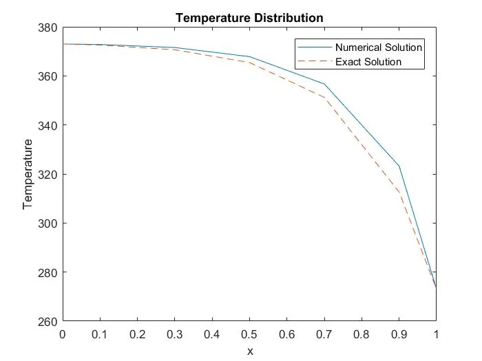

3)u=2.5m/s
The system goes into a infinite loop and does not return with a solution.

Lets find u=2.5m/s for n=10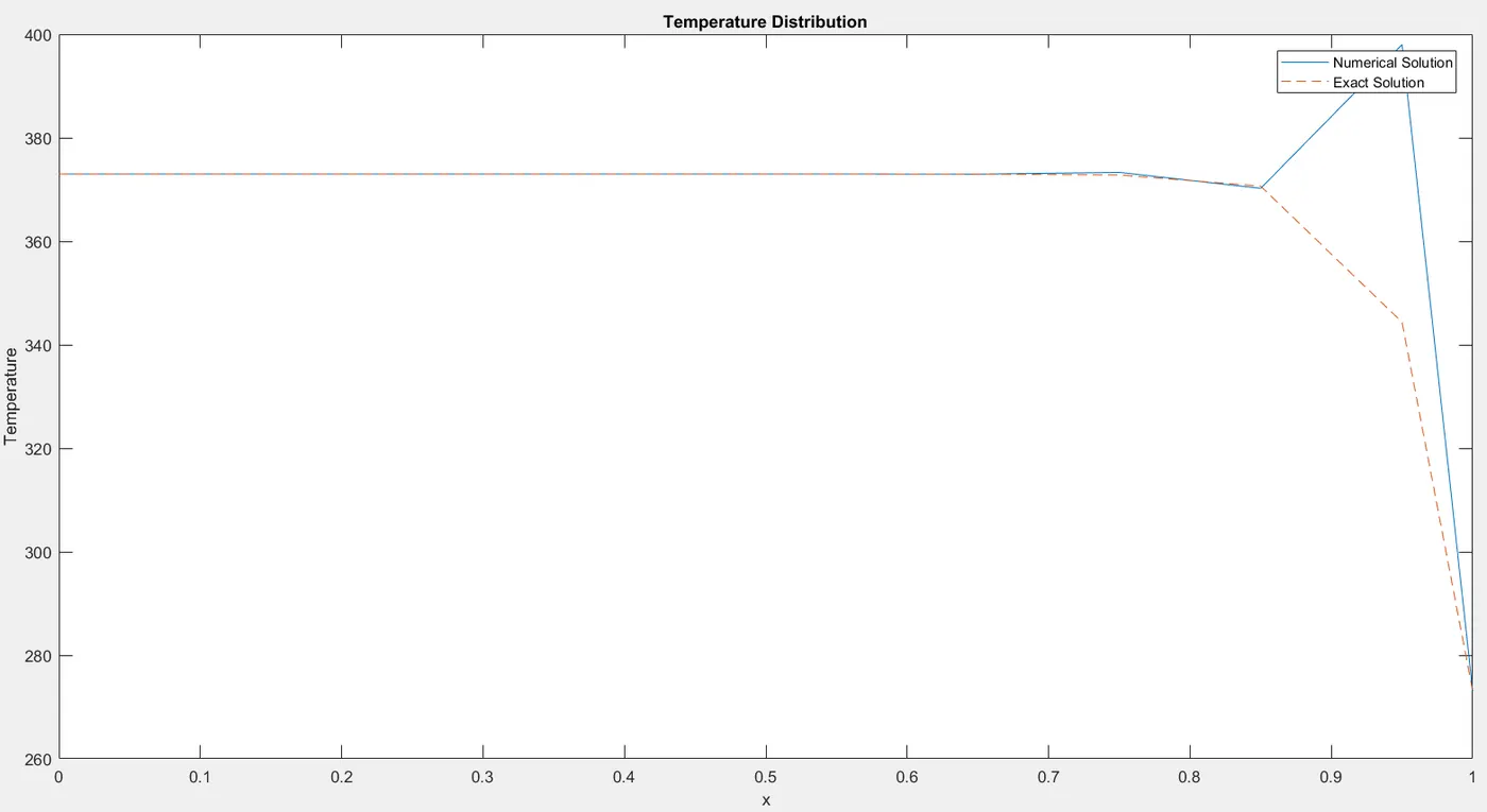


Assessment of the method:-
i) Conservativeness
The numerical governing equation for a control volume
`F_ephi_e-F_wphi_w=D_e(phi_E-phi_P)-D_w(phi_P-phi_W)`
Now rearranging it we get
`F_wphi_w-D_w(phi_P-phi_W)=F_ephi_e-D_e(phi_E-phi_P)`
From the above equation
we find
Flux entering via west face=flux leaving out of east face
`q_w=q_e`
Now since flux of scalar quantity entering west face is not lost while it passes through east face, this means the scalar quantity is conserved.

ii)Boundedness
It means whether the system of equations in the scalar quantities will converge towards a solution or not.
Scarborough (1958) gave a condition to check whether the system of equation is converging or not.
The condition is
`sumabs(a_(nb))/abs(a_(p)) {(<=,1,at,all,nodes),(<,1,at,a,node):}`
This means that in the absence of Sources the internal node values of property `phi` should be bounded by boundary values.

iii)Transportiveness
The transportiveness property of a fluid flow can be illustrated by a non-dimensional number called Peclet number
Peclet number=`Pe=F/D=(rho u)/(Gamma/(delx))`
this number measures the relative strengths of convection and diffusion.
`delx`is the characteristics length of the cell or control Volume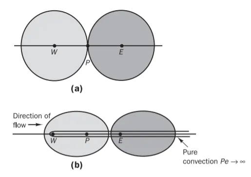

This is extract from An Introduction to Computational Fluid Dynamics by H K Versteeg and W Malalasekera
In the image 2 cases have been shown of influence of scalar field `phi`between different nodes due to diffusion and convection.
Case-a:- Its a case of pure Diffusion, in such a case scalar field value at W and E will have equal effect on node P.
In this case, Pe=0
Case-b:- Its a case of pure convection, in such case only scalar field value at W(node upstream) will have influence at node P and not that from node E. In such a case any equation solved from equal contribution from both east and west face fails to converge.

That is why when u=2.5m/s and dx is little large, so that influence due to convection increases from a upstream face and consequently decreases significantly from east face. That is why the system of equation fails. So by decreasing dx value, thereby decreasing Peclet number and convection influence makes the system convergent again.

2) Upwind Differencing Scheme

So here the interpolation is done as
When u>0
`phi_w=phi_W`
`phi_e=phi_P`
And when u<0
`phi_w=phi_P`
`phi_e=phi_E`
So basically the value at a wall of a control volume is the value of central node of a control volume upstream of the flow at that wall.
Lets substitute in the convective flux side of the equation
`(del(rhophiu))/(delx)|_P=(F_ephi_P-F_wphi_W)/dx`
This on further simplification becomes
`(del(rhophiu))/(delx)|_P=F(phi_P-phi_W)/dx=F(phi_i-phi_(i-1))/dx`
This as it can be seen becomes the first order approximation of first order derivative. Because of it being first order, it gives rise to false diffusion effect which will slowly decrease the intensity of solution as it converges depending on the decretization interval dx.
Like done for central difference scheme, in this scheme as well respective substitutions will be made in the main governing numerical equation.
So after substitution main governing equation becomes
So when u>0
`F_ephi_P-F_wphi_W=D_e(phi_E-phi_P)-D_w(phi_P-phi_W)`
when u<0
`F_ephi_E-F_wphi_P=D_e(phi_E-phi_P)-D_w(phi_P-phi_W)`
So after rearranging above equation, it can be generalized as
`a_Pphi_P=a_Wphi_W+a_Ephi_E`
`a_W=D_w+max(F_w,0)=D_w+alpha_wF_w`
`a_E=De+max(0,-Fe)=De-(1-alpha_e)*F_e`
`a_P=a_W+a_E+Fe-Fw`

Note:-
From here on wherever `alpha` will be used, its value is determined by direction of u.
If u>0,`alpha=1`
If u<0,`alpha=0`

Now as conditioning to the equation was done for border nodes in central differencing scheme, it will be required for this scheme as well.
when u>0
For node 1,
`F_ephi_P-F_AphiA=D_e(phi_E-phi_P)-D_A(phi_P-phi_A)`
For node 5,
`F_BphiB-F_wphi_W=D_B(phiB-phi_P)-D_w(phi_P-phi_W)`
Now rearranging the above equation and repeating the same exercise for u<0, the equation can be generalised for all points in the domain as
`a_Pphi_P=a_Wphi_W+a_Ephi_E+Su`
`a_P=a_W+a_E+Sp+Fe-Fw`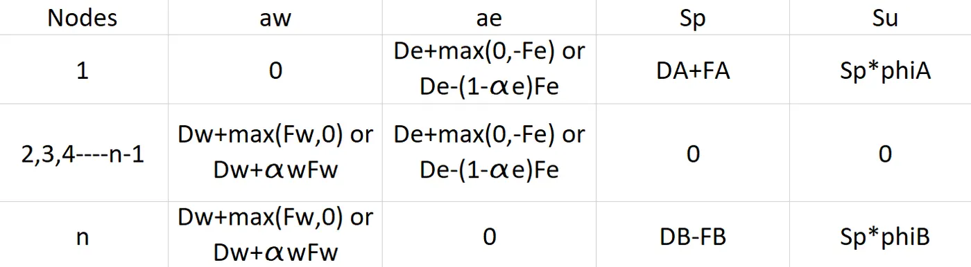

Remember DA=DB=2D and FA=FB=F
Now this generalised equation is transformed into a code and problem is solved for the sample situation of fluid as done for central difference scheme.
The code is solved using gauss seidel iterative solver

clear all
close all
clc
%Input

n=5;
L=1;%in meter
rho=1;%kg/m^3
T=0.1;
u=0.1;%m/s

%Derived Values

F=rho*u;
dx=L/n;
D=T/dx;
nx=n+2;% Position number

%Domain

x(1)=0;
x(2:nx-1)=(dx/2):dx:(L-(dx/2));
x(nx)=L;

%Initial Output

phiA=373;
phiB=273;
phi=zeros(1,nx);
phi(1)=phiA;
phi(nx)=phiB;

%Iteration Settings

tol=1e-5;
error=9e9;

%Solver
while(error>tol)
phiold=phi;
for i=2:nx-1
if i==2
   aw=0;
   Aw=0;
   Sp=2*D+F;
   Su=Sp*phiA;
else
   aw=D+max([F 0]);
   Aw=aw*phi(1,i-1);
end
if i==(nx-1)
   ae=0;
   Ae=0;
   Sp=2*D-F;
   Su=Sp*phiB;
else
   ae=D+max([-F 0]);
   Ae=ae*phiold(1,i+1);
end
if i~=2
  if i~=nx-1
Sp=0;
Su=0;
  end
end
ap=aw+ae+Sp;
phi(1,i)=(Ae+Aw+Su)/ap;  
end
error=max(abs(phi-phiold));
end
[phi_exact]=Exact_diffusion_Convection_Solver(rho,u,T,phiA,phiB,x);
plot(x,phi)
hold on
plot(x,phi_exact,'--')
xlabel('x')
ylabel('Temperature')
title('Temperature Distribution')
legend('Numerical Solution','Exact Solution')

when n=5
1) u=0.1m/s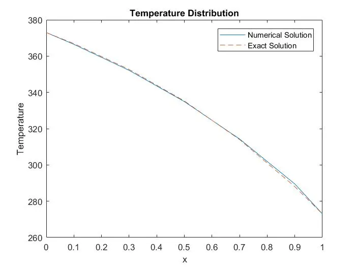

2) u=0.5m/s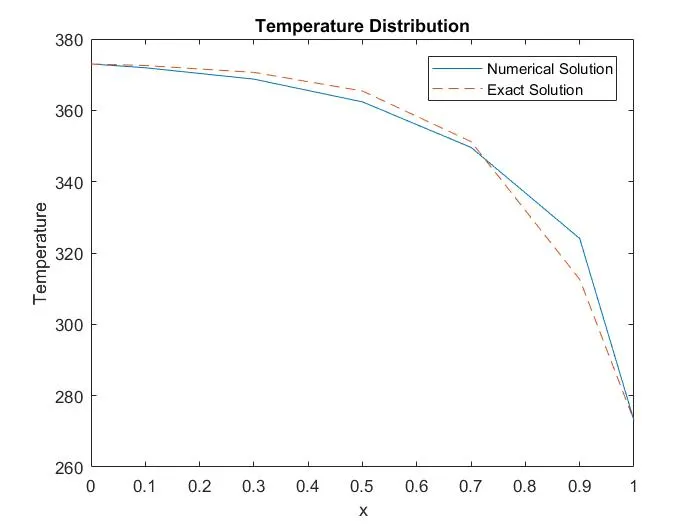
3) u=2.5m/s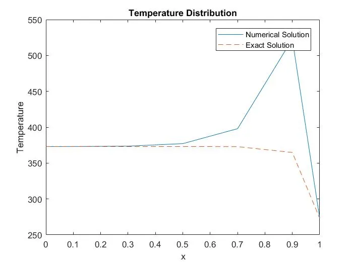

when n=10, u=2.5m/s

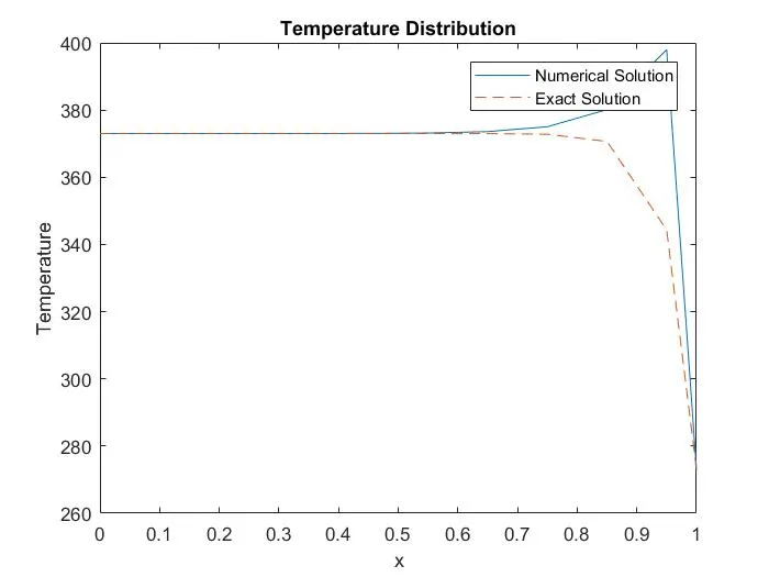
Assessment:-

Conservativeness:
the expressions are consistent in this scheme which are used to calculate flux and hence they are conservative.

Boundedness:-
Now it is found that `a_P`is always greater than `a_W`and `a_E`, since there are no negative terms in `a_P`whether the flow is negative or positive. Hence the iterative solution will always converge. Therefore the scheme is bounded.

Transportiveness:-
Now if central differencing and upward differencing are compared, the solution converges for n=5 and u=2.5m/s for upwind and not for central. this happens because, upwind method assigns more importance to terms upwind to the fluid flow than that in downwind. This means when u value becomes high, then diffusive effect becomes inconsequential and convective effect became more dominant. This is the reason why at higher value of u, values from terms upwind are necessary and not from that in downwind.

Accuracy:-
Now difference in accuracy is much more fathomable for u=0.5 and n=5 for both central difference and upwind scheme. As it can be observed that the accuracy or fit to the exact curve is better for central difference scheme and less for upwind difference scheme. This is due to false diffusion effect in upwind differencing scheme.

Stability:-
Though it is true that solution converges for n=5 and u=2.5m/s for upwind and not for central. Both show wiggles or upshoots, when n=10 with u=2.5m/s and both converge. But central difference will tend to wiggle more than the other.

3) Hybrid Differencing Scheme

Now looking at central differencing scheme and understand it further,
lets understand flux of`phi`through west face due to convection and diffusion,
`q_w=F_wphi_w-D_w(phi_P-phi_W)`
substituting the scheme, we get
`q_w=F_w(phi_W+phi_P)/2-D_w(phi_P-phi_W)`
Rearranging we get
`q_w=(F_w/2+D_w)phi_W+(F_w/2-D_w)phi_P`
Now taking out `F_w/2`out from the equation as a factor we get
`q_w=F_w/2((1+2(D_w/F_w))phi_W+(1-2(D_w/F_w))phi_P)`
but we know that Peclet number is `Pe_w=F_w/D_w`
Making the substitution in the above equation,
`q_w=F_w/2((1+2/(Pe_w))phi_W+(1-2/(Pe_w))phi_P)`
Now looking at the equation, if `Pe>=2`,`phi_W`becomes dominant and `phi_P`values effect will becomes inconsequential. And if `Pe_w<=-2`, `phi_P`becomes dominant and`phi_W`values effect will becomes inconsequential.
So central differencing scheme is best for `abs(Pe_w)<2`
And upwind differencing scheme is best for `abs(Pe_w)>=2`

The hybrid differencing scheme of Spalding (1972) is based on a combination of central and upwind differencing schemes. So The hybrid differencing scheme uses piecewise formulae based on the local Peclet number to evaluate the net flux through each control volume face. It utilizes the best of both schemes.

So for `abs(Pe_w)<2`
`q_w=F_w/2((1+2/(Pe_w))phi_W+(1-2/(Pe_w))phi_P)`
And for `abs(Pe_w)>=2`, applying upwind scheme
when `Pe_w>=2`
`q_w=F_wphi_W`+ Diffusion effect neglected
when `Pe_w<=-2`
`q_w=F_wphi_P`+Diffusion effect neglected

So after generalization of equation for nodes and border conditioning, a general equation is devised as follows
`a_Pphi_P=a_Wphi_W+a_Ephi_E+Su`
`a_P=a_W+a_E+Sp+Fe-Fw`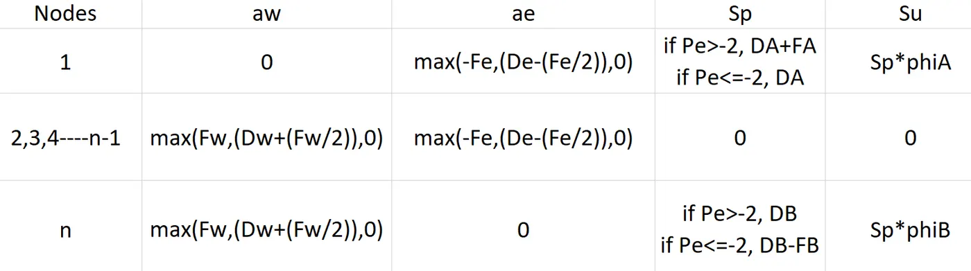


Note:- Now it is understood that when `abs(Pe)>=2`, though diffusion effect is taken as zero but is considered for border nodes to take into information from domain boundary value even when convective effect does not carry that information to the system. For example if Pe>2 this means that u>2, therefore at boundary node n, `phi_e=phi_P!=phiB` so what happens that the value of phi_B does not reach the system through out the calculation. this is the reason diffusive effect is accounted for at border nodes when it is not done for other nodes.

Now this generalized equation is transformed into a code and gauss-seidel solver is used to solve the system.

clear all
close all
clc
%Input

n=5;
L=1;%in meter
rho=1;%kg/m^3
T=0.1;
u=0.1;%m/s

%Derived Values

F=rho*u;
dx=L/n;
D=T/dx;
Pe=F/D;
nx=n+2;% Position number

%Domain

x(1)=0;
x(2:nx-1)=(dx/2):dx:(L-(dx/2));
x(nx)=L;

%Initial Output

phiA=373;
phiB=273;
phi=zeros(1,nx);
phi(1)=phiA;
phi(nx)=phiB;

%Iteration Settings

tol=1e-4;
error=9e9;

%Solver
while(error>tol)
phiold=phi;
for i=2:nx-1
if i==2
   aw=0;
   Aw=0;
  if Pe>-2
   Sp=2*D+F;
  else
   Sp=2*D;
  end
   Su=Sp*phiA;
else
   aw=max([F D+(F/2) 0]);
   Aw=aw*phi(1,i-1);
end
if i==(nx-1)
   ae=0;
   Ae=0;
  if Pe>-2
   Sp=2*D;
  else
   Sp=2*D-F;
  end
   Su=Sp*phiB;
else
   ae=max([0 -F D-(F/2)]);
   Ae=ae*phiold(1,i+1);
end
if i~=2
  if i~=nx-1
Sp=0;
Su=0;
  end
end
ap=aw+ae+Sp;
phi(1,i)=(Ae+Aw+Su)/ap;  
end
error=max(abs(phi-phiold));
end
[phi_exact]=Exact_diffusion_Convection_Solver(rho,u,T,phiA,phiB,x);
plot(x,phi)
hold on
plot(x,phi_exact,'--')
xlabel('x')
ylabel('Temperature')
title('Temperature Distribution')
legend('Numerical Solution','Exact Solution')

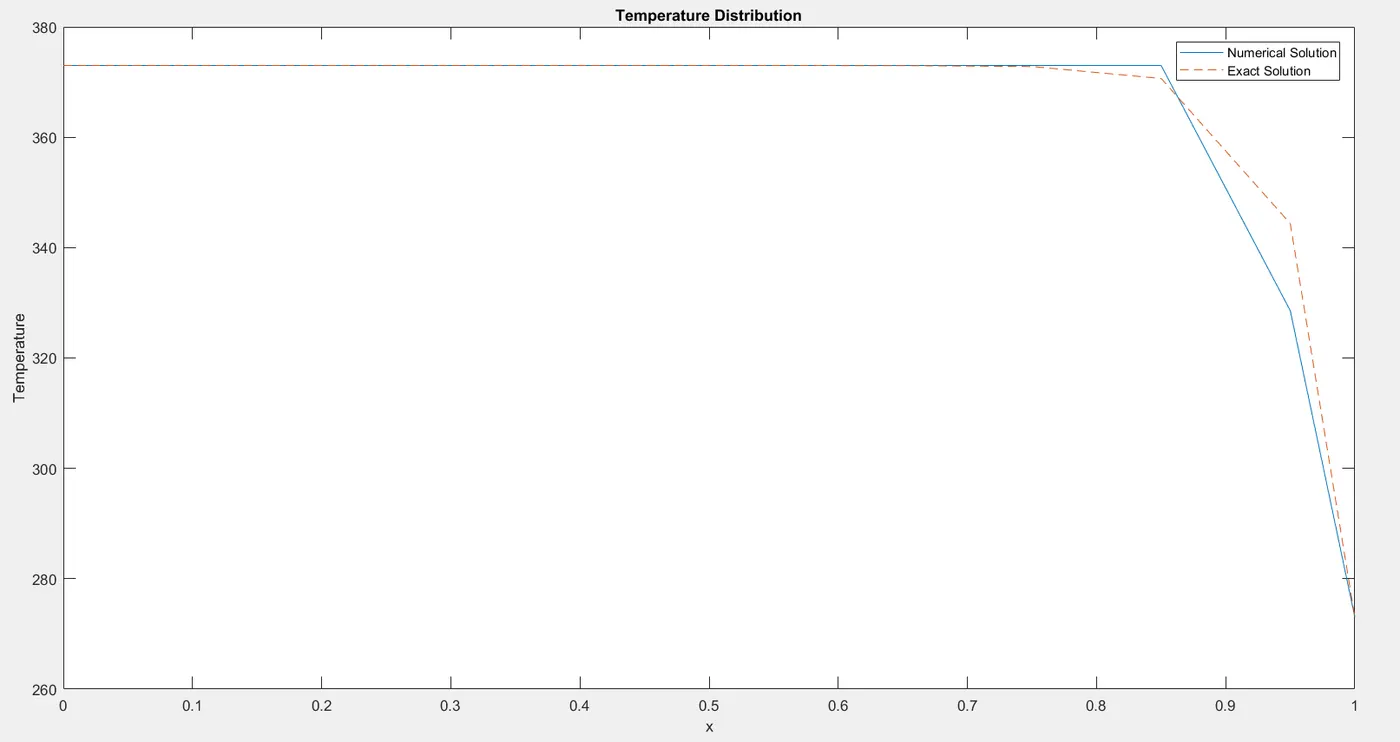
When n=5
i) u=0.1m/s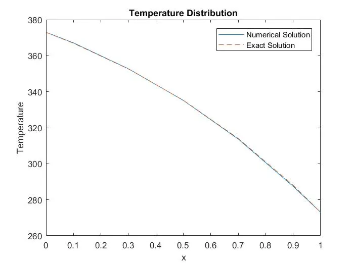

ii)u=0.5 m/s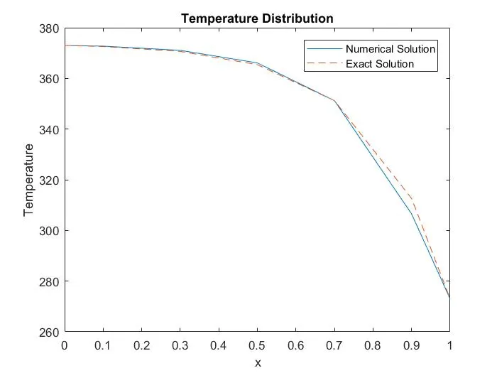

iii)u=2.5m/s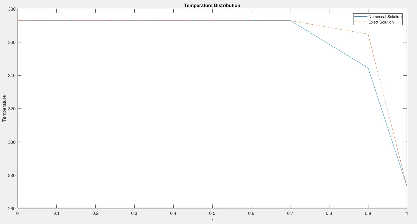

when n=10 and u=2.5 m/s


Assessment of hybrid differencing method
The hybrid difference scheme exploits the favourable properties of the
upwind and central differencing schemes
1)The scheme is fully conservative and since the coefficients are always positive it is unconditionally bounded.
2) It switches to upwind differencing when central differencing produces inaccurate results at high Pe numbers.Hence it satisfies the transportiveness requirement by using an upwind formulation for large values of Peclet number.
3) Stability:- Compare u=25 for n=5 and 10, for central and upwind differencing scheme with that of hybrid differencing scheme. It is found that there are no upshoots for hybrid unlike that in central and upwind schemes. Hence it is more stable. It is said to be even more stable than QUICK scheme.
4) Accuracy:- Its just that its trucation error is of first order when `abs(Pe)>=2`. This leads to false diffusion to some extent. Though this scheme is more accurate than central and upwind scheme, as can be observed on comparison between results obtained for n=5 and u=0.5m/s.
5)It is used in lot many CFD application.

4) The Power Law scheme

The power-law differencing scheme of Patankar (1980) is a more accurate approximation to the one-dimensional exact solution and produces better results than the hybrid scheme. In this scheme diffusion is set to zero when cell Pe exceeds 10. If 0 < Pe < 10 the flux is evaluated by using a polynomial expression.

In this the net flux through west face is given by
`q_w=F_w[phi_W-beta_w(phi_P-phi_W)]` for 0<Pe<10
where `beta_w=(1-0.1Pe_w)^5/(Pe_w)`
`q_w=F_wphi_W`+ diffusion effect neglected for Pe>10

Now after generalization and border node conditioning, we get
`a_Pphi_P=a_Wphi_W+a_Ephi_E+Su`
`a_P=a_W+a_E+Sp+Fe-Fw`

Note:- Now it is understood that when `abs(Pe)>=10`, though diffusion effect is taken as zero but is considered for border nodes to take into information from domain boundary value even when convective effect does not carry that information to the system. For example if Pe>10 this means that u>0, therefore at boundary node n, `phi_e=phi_P!=phiB` so what happens that the value of phi_B does not reach the system through out the calculation. This is the reason diffusive effect is accounted for at border nodes when it is not done for other nodes.

Now this generalized equation will be transformed into a code and solved using gauss seidel iterative solver.

clear all
close all
clc
%Input

n=5;
L=1;%in meter
rho=1;%kg/m^3
T=0.1;
u=0.1;%m/s

%Derived Values

F=rho*u;
dx=L/n;
D=T/dx;
Pe=F/D;
nx=n+2;% Position number

%Domain

x(1)=0;
x(2:nx-1)=(dx/2):dx:(L-(dx/2));
x(nx)=L;

%Initial Output

phiA=373;
phiB=273;
phi=zeros(1,nx);
phi(1)=phiA;
phi(nx)=phiB;

%Iteration Settings

tol=1e-4;
error=9e9;

%Solver
while(error>tol)
phiold=phi;
for i=2:nx-1
if i==2
   aw=0;
   Aw=0;
  if -10>Pe
   Sp=2*D;
  elseif Pe>=-10 && 10>=Pe
   Sp=2*D*((1-0.1*abs(Pe))^5)+max([F 0]);
  else
   Sp=2*D+F;
  end
   Su=Sp*phiA;
else
   aw=D*max([0 ((1-0.1*abs(Pe))^5)])+max([F 0]);
   Aw=aw*phi(1,i-1);
end
if i==(nx-1)
   ae=0;
   Ae=0;
  if -10>Pe
   Sp=2*D-F;
  elseif Pe>=-10 && 10>=Pe
   Sp=2*D*((1-0.1*abs(Pe))^5)+max([-F 0]);
  else
   Sp=2*D;
  end
   Su=Sp*phiB;
else
   ae=D*max([0 ((1-0.1*abs(Pe))^5)])+max([-F 0]);
   Ae=ae*phiold(1,i+1);
end
if i~=2
  if i~=nx-1
Sp=0;
Su=0;
  end
end
ap=aw+ae+Sp;
phi(1,i)=(Ae+Aw+Su)/ap;  
end
error=max(abs(phi-phiold));
end
[phi_exact]=Exact_diffusion_Convection_Solver(rho,u,T,phiA,phiB,x);
plot(x,phi)
hold on
plot(x,phi_exact,'--')
xlabel('x')
ylabel('Temperature')
title('Temperature Distribution')
legend('Numerical Solution','Exact Solution')

when n=5
i) u=0.1m/s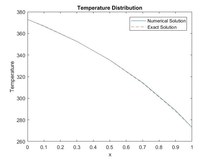

ii)u=0.5 m/s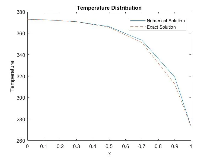

iii)u=2.5 m/s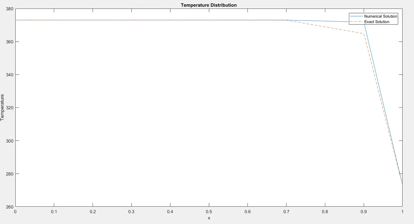

when n=10 and u=2.5m/s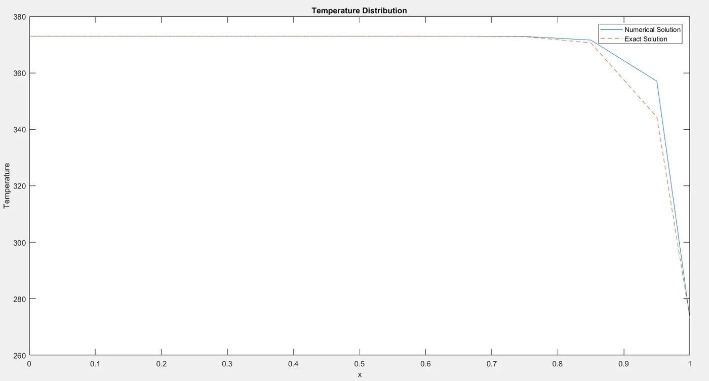


Assessment of Power law scheme
Properties of the power-law differencing scheme are similar to those of the hybrid scheme. The power-law differencing scheme is more accurate for one-dimensional problems since it attempts to represent the exact solution more closely. The scheme has proved to be useful in practical flow calculations and can be used as an alternative to the hybrid scheme. It is also as stable as hybrid scheme.

Higher order Schemes

1)Upwind and Hybrid schemes are first order schemes and though they are stable, scheme leads to false diffusion in the solution.
2)Central Differencing has a second order accuracy but is unstable on certain accounts and does not possess transportativesness property

So to counter this, more than one point is taken to increase the accuracy and the numerical scheme is left skewed which mimics upwind scheme in terms of stability. So lets start with oldest of these higher-order schemes- Leonard's QUICK scheme

5) QUICK (Quadratic Upstream Interpolation for Convective Kinetics)

It uses a three-point weighted quadratic interpolation for cell values:- A node on either sides of present node (P) i.e West node (W) and East node (E) and node further upstream if u>0 :- WW or if u<0 :- EE
when u>0,
`phi_w=(6/8)phi_W+(3/8)phi_P-(1/8)phi_(WW)`
`phi_e=(6/8)phi_P+(3/8)phi_E-(1/8)phi_(W)`
when u<0
`phi_w=(6/8)phi_P+(3/8)phi_W-(1/8)phi_(E)`
`phi_e=(6/8)phi_E+(3/8)phi_P-(1/8)phi_(E E)`
Now we know that the governing numerical equation is
`F_ephi_e-F_wphi_w=D_e(phi_E-phi_P)-D_w(phi_P-phi_W)`
So when u>0
`F_e((6/8)phi_P+(3/8)phi_E-(1/8)phi_(W))-F_w((6/8)phi_W+(3/8)phi_P-(1/8)phi_(WW))=D_e(phi_E-phi_P)-D_w(phi_P-phi_W)`
And when u<0
`F_e((6/8)phi_E+(3/8)phi_P-(1/8)phi_(E E))-F_w((6/8)phi_P+(3/8)phi_W-(1/8)phi_(E))=D_e(phi_E-phi_P)-D_w(phi_P-phi_W)`
Now an important notice is that, for border node conditioning
`Gamma(dphi)/(dx)|_A=(DA)/3(9phi_P-8phiA-phi_E)!=DA(phi_P-phiA)` unlike in previous schemes
and DA=D or `DA!=2D` unlike in previous schemes
Similarly for
node n
`Gamma(dphi)/(dx)|_B=(DB)/3(8phiB-9phi_P+phi_W)!=DB(phi_P-phiB)`
and `DB=D!=2D`

Now numerical governing equation
for u>0
1)Node 1
`F_e((6/8)phi_P+(3/8)phi_E-(1/8)phi_(W))-F_AphiA=D_e(phi_E-phi_P)-(DA)/3(9phi_P-8phiA-phi_E)`
2)Node n
`FBphiB-F_w((6/8)phi_W+(3/8)phi_P-(1/8)phi_(WW))=(DB)/3(8phiB-9phi_P+phi_W)-D_w(phi_P-phi_W)`
for u<0
1)Node 1
`F_e((6/8)phi_E+(3/8)phi_P-(1/8)phi_(E E))-F_AphiA=D_e(phi_E-phi_P)-(DA)/3(9phi_P-8phiA-phi_E)`
2)Node n
`FBphiB-F_w((6/8)phi_P+(3/8)phi_W-(1/8)phi_(E))=(DB)/3(8phiB-9phi_P+phi_W)-D_w(phi_P-phi_W)`
Now conditioning of border nodes is done by rearranging of the above equations and generalizing them, the domain boundary values phiA and phiB are also found to mirror values of `phi_(WW)`and `phi_(E E)` respectively for nodes 2 and n-1 respectively. So conditioning of the 2 and n-1 node equation also need to be done by substituting
for node 2
`phi_(WW)=2phiA-phi_W`
for node 3
`phi_(E E)=2phiB-phi_(E)`
Substituting the above expressions in numerical governing equation for node 2 and node n-1, we will get governing equation for those nodes.
Now after intense calculation and generalization, a general equation is obtained to encompasse all the nodes in the domain.
`a_Pphi_P=a_(WW)phi_(WW)+a_Wphi_W+a_Ephi_E+a_(E E)phi_(E E)+Su`
`a_P=a_(WW)+a_W+a_E+a_(E E)+Sp+Fe-Fw`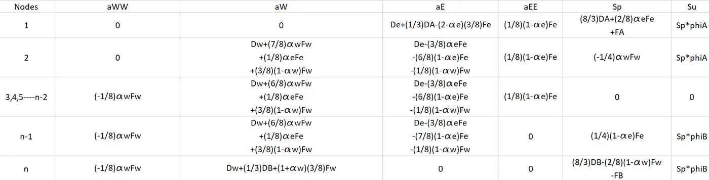

Now this generalized equation will be transformed into a code and solved using jacobi iterative solver.

clear all
close all
clc
%Input

n=10;
L=1;%in meter
rho=1;%kg/m^3
T=0.1;
u=2.5;%m/s

%Derived Values

F=rho*u;
dx=L/n;
D=T/dx;
nx=n+2;% Position number
if u>=0
alpha=1;
else
alpha=0;
end
%Domain

x(1)=0;
x(2:nx-1)=(dx/2):dx:(L-(dx/2));
x(nx)=L;

%Initial Output

phiA=373;
phiB=273;
phi=zeros(1,nx);
phi(1)=phiA;
phi(nx)=phiB;

%Iteration Settings

tol=1e-5;
error=9e9;

%Solver
while(error>tol)
phiold=phi;
for i=2:nx-1
if i==2
aww=0;
Aww=0;
aw=0;
Aw=0;
ae=D+(1/3)*D-(2-alpha)*(3/8)*F;
Ae=ae*phiold(1,i+1);
aee=(1/8)*(1-alpha)*F;
Aee=aee*phiold(1,i+2);
Sp=(8/3)*D+(2/8)*F*alpha+F;
Su=Sp*phiA;
elseif i==3
aww=0;
Aww=0;
aw=D+(7/8)*alpha*F+(1/8)*alpha*F+(3/8)*(1-alpha)*F;
Aw=aw*phiold(1,i-1);
ae=D-(3/8)*alpha*F-(6/8)*(1-alpha)*F-(1/8)*(1-alpha)*F;
Ae=ae*phiold(1,i+1);
aee=(1/8)*(1-alpha)*F;
Aee=aee*phiold(1,i+2);
Sp=-(1/4)*alpha*F;
Su=Sp*phiA;
elseif i==nx-2
aww=-alpha*(1/8)*F;
Aww=aww*phiold(1,i-2);
aw=D+(3/8)*(1-alpha)*F+(6/8)*alpha*F+(1/8)*alpha*F;
Aw=aw*phiold(1,i-1);
ae=D-(7/8)*(1-alpha)*F-(1/8)*(1-alpha)*F-(3/8)*alpha*F;
Ae=ae*phiold(1,i+1);
aee=0;
Aee=0;
Sp=(1/4)*(1-alpha)*F;
Su=Sp*phiB;
elseif i==nx-1
aww=-alpha*(1/8)*F;
Aww=aww*phiold(1,i-2);
aw=D+(1/3)*D+(1+alpha)*(3/8)*F;
Aw=aw*phiold(1,i-1);
ae=0;
Ae=0;
aee=0;
Aee=0;
Sp=(8/3)*D-(2/8)*F*(1-alpha)-F;
Su=Sp*phiB;
else
aww=-alpha*(1/8)*F;
Aww=aww*phiold(1,i-2);
aw=D+(3/8)*(1-alpha)*F+(6/8)*alpha*F+(1/8)*alpha*F;
Aw=aw*phiold(1,i-1);
ae=D-(3/8)*alpha*F-(6/8)*(1-alpha)*F-(1/8)*(1-alpha)*F;
Ae=ae*phiold(1,i+1);
aee=(1/8)*(1-alpha)*F;
Aee=aee*phiold(1,i+2);
Sp=0;
Su=0;
end
ap=aww+aw+ae+aee+Sp;
phi(1,i)=(Aww+Aw+Ae+Aee+Su)/ap;  
end
error=max(abs(phi-phiold));
end
[phi_exact]=Exact_diffusion_Convection_Solver(rho,u,T,phiA,phiB,x);
plot(x,phi)
hold on
plot(x,phi_exact,'--')
xlabel('x')
ylabel('Temperature')
title('Temperature Distribution')
legend('Numerical Solution','Exact Solution')

when n=5,
i)u=0.1m/s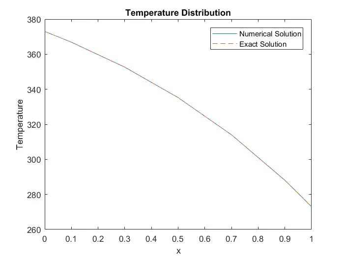

ii)u=0.5m/s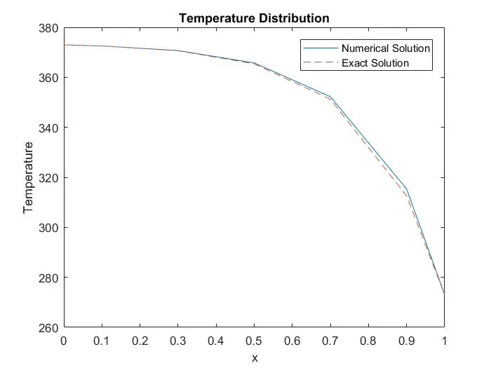

iii)u=2.5m/s
The solution did not converge for n=5 and u=2.5m/s
when n=10 and u=2.5m/s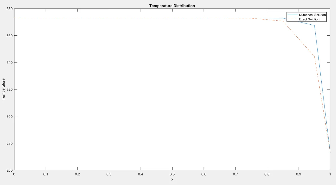


Assessment of QUICK method:-
1) The terms are consisteny and therefore the scheme is conservative.
2) Since the scheme is based on a quadratic function its accuracy in terms of Taylor series
truncation error is third-order on a uniform mesh.
3)The transportiveness property is built into the scheme as the quadratic function is based on two upstream and one downstream nodal values.
4)The main coefficients (E and W) are not guaranteed to be positive and the coefficients `a_(WW)` and `a_(E E)` are negative. For example, if uw > 0 and ue > 0 the east coefficient becomes negative at relatively modest cell Peclet numbers (Pee = Fe/De > 8/3). As it can be observed that for u=2.5m/s and n=5, the system does not converge. This happens because of the negative terms.

To counter Leonard's QUICK scheme's disadvantage in stability, Hayase(1992) QUICK scheme is to be implemented.

Hayase's QUICK scheme

Now what Hayase did was he converted the QUICK equation into a upwind equation with a source term.
`a_(P_(UW))phi_P=a_(W_(UW))phi_W+a_(E_(UW))phi_E+bar S`
`a_(P_(UW))=a_(W_(UW))+a_(E_(UW))+Fe-Fw`
UW stands for Upwind

And the table given for these variables above is given in An Introduction to Computational Fluid Dynamics by H K Versteeg and W Malalasekera.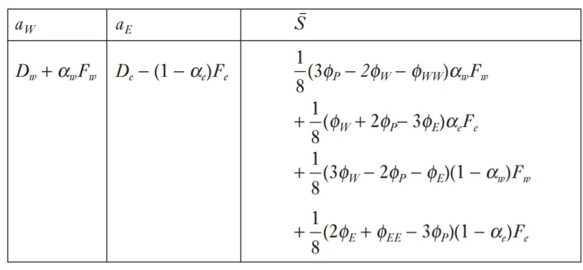

But the generalization does not solve here, border conditioning is required. For this no formula is given in the book.
Now on little investigation a finding was made. To make it clear, something need to be specified:-
Let us first put forth Leonard's QUICK method (for which value was given in a table previously)
`a_Pphi_P=a_(WW)phi_(WW)+a_Wphi_W+a_Ephi_E+a_(E E)phi_(E E)+Su`
`a_P=a_(WW)+a_W+a_E+a_(E E)+Sp+Fe-Fw`
while the above same equation is transformed into a equation system as follows
`a_(P_(UW))phi_P=a_(W_(UW))phi_W+a_(E_(UW))phi_E+bar S`....`Su_(UW)`is included in `barS`
`a_(P_(UW))=a_(W_(UW))+a_(E_(UW))+Sp_(UW)+Fe-Fw`....`Sp_(UW)` is from Sp of Upwind equation
Now we have expressions `a_(P_(UW)),a_(W_(UW)),a_(E_(UW)) and Sp_(UW)`from Upwind differencing scheme and `a_P,a_(WW),a_W,a_E,a_(E E) and Sp`from Leonard's QUICK scheme which were derived previously.
It was found for a general node (not considering terms such as `Sp_(UW),Su_(UW),Sp and Su`) that
`barS=(phi_W-phi_P)Deltaa_W+(phi_E-phi_P)Deltaa_E+(phi_(WW)-phi_P)a_(WW)+(phi_(E E)-phi_P)a_(E E)`
where `Deltaa_W=a_W-a_(W_(UW))`
`Deltaa_E=a_E-a_(E_(UW))`
Now this expression was found to be true with the value of expression given by H K Versteeg and W Malalasekera (in the table).

Now a complete generalization for all the nodes including one at the border is as follows based on the finding above:-
`a_(P_(UW))phi_P=a_(W_(UW))phi_W+a_(E_(UW))phi_E+bar S`
`a_(P_(UW))=a_(W_(UW))+a_(E_(UW))+Sp_(UW)+Fe-Fw`
Now in the above equation, except `bar S`every term can be obtained from the table of terms developed for Upwind scheme.
The expression for `bar S`including the terms for border nodes are:-
`barS=(phi_W-phi_P)Deltaa_W+(phi_E-phi_P)Deltaa_E+(phi_(WW)-phi_P)a_(WW)+(phi_(E E)-phi_P)a_(E E)-DeltaSpphi_P+Su`
where `Deltaa_W=a_W-a_(W_(UW))`
`Deltaa_E=a_E-a_(E_(UW))`
`DeltaSp=Sp-Sp_(UW)`
where `a_P,a_(WW),a_W,a_E,a_(E E),Sp and Su`from Leonard's QUICK scheme derived in the table in the previous section.

Now that generalization of equation is done, lets understand the reason why `bar S`was taken to seperate location in an otherwise Leonard's QUICK scheme equation.
It was found that due to negative terms in expressions for `a_W and a_E`plunged the system of equation into non-convergence. So to counter this `bar S`was created to accumulating all the expressions which were negative and to make the main expressions that of Upwind scheme. This `bar S`is called delayed correction term. Because the `phi`terms value is put that of previous iteration. So it is found that this delayed correction eventually catches up to increase the accuracy in an otherwise solution of upwind scheme and make the solution as accurate as in Leonard's scheme minus the stability problem in that.
This generalisation of equation was converted into a code and solved using Jacobi iterative solver.

clear all
close all
clc
%Input

n=5;
L=1;%in meter
rho=1;%kg/m^3
T=0.1;
u=2.5;%m/s

%Derived Values

F=rho*u;
dx=L/n;
D=T/dx;
nx=n+2;% Position number
if u>=0
alpha=1;
else
alpha=0;
end
%Domain

x(1)=0;
x(2:nx-1)=(dx/2):dx:(L-(dx/2));
x(nx)=L;

%Initial Output

phiA=373;
phiB=273;
phi=zeros(1,nx);
phi(1)=phiA;
phi(nx)=phiB;

%Iteration Settings

tol=1e-5;
error=9e9;
%Solver
while(error>tol)
phiold=phi;
for i=2:nx-1
if i==2
   %Upwind Scheme Terms
   aw_uw=0;
   Aw=0;
   ae_uw=D-(1-alpha)*F;
   Ae=ae_uw*phiold(1,i+1);
   Sp_uw=2*D+F;
   %QUICK scheme terms
   aww=0;
   Saww=0;
   aee=(1/8)*(1-alpha)*F;
   Saee=(phiold(1,i+2)-phiold(1,i))*aee;
   aw=0;
   d_aw=aw-aw_uw;
   Saw=0;
   ae=D+(1/3)*D-(2-alpha)*(3/8)*F;
   d_ae=ae-ae_uw;
   Sae=(phiold(1,i+1)-phiold(1,i))*d_ae;
   Sp=(8/3)*D+(2/8)*F*alpha+F;
   d_sp=Sp-Sp_uw;
   Ssp=d_sp*phiold(1,i);
   Su=Sp*phiA;
elseif i==3
   %Upwind Scheme Terms
   aw_uw=D+alpha*F;
   Aw=aw_uw*phiold(1,i-1);
   ae_uw=D-(1-alpha)*F;
   Ae=ae_uw*phiold(1,i+1);
   Sp_uw=0;
   %QUICK scheme terms
   aww=0;
   Saww=0;
   aee=(1/8)*(1-alpha)*F;
   Saee=(phiold(1,i+2)-phiold(1,i))*aee;
   aw=D+(7/8)*alpha*F+(1/8)*alpha*F+(3/8)*(1-alpha)*F;
   d_aw=aw-aw_uw;
   Saw=(phiold(1,i-1)-phiold(1,i))*d_aw;
   ae=D-(3/8)*alpha*F-(6/8)*(1-alpha)*F-(1/8)*(1-alpha)*F;
   d_ae=ae-ae_uw;
   Sae=(phiold(1,i+1)-phiold(1,i))*d_ae;
   Sp=-(1/4)*alpha*F;
   d_sp=Sp-Sp_uw;
   Ssp=d_sp*phiold(1,i);
   Su=Sp*phiA;
elseif i==nx-2
   %Upwind Scheme Terms
   aw_uw=D+alpha*F;
   Aw=aw_uw*phiold(1,i-1);
   ae_uw=D-(1-alpha)*F;
   Ae=ae_uw*phiold(1,i+1);
   Sp_uw=0;
   %QUICK scheme terms
   aww=-alpha*(1/8)*F;
   Saww=(phiold(1,i-2)-phiold(1,i))*aww;
   aee=0;
   Saee=0;
   aw=D+(3/8)*(1-alpha)*F+(6/8)*alpha*F+(1/8)*alpha*F;
   d_aw=aw-aw_uw;
   Saw=(phiold(1,i-1)-phiold(1,i))*d_aw;
   ae=D-(7/8)*(1-alpha)*F-(1/8)*(1-alpha)*F-(3/8)*alpha*F;
   d_ae=ae-ae_uw;
   Sae=(phiold(1,i+1)-phiold(1,i))*d_ae;
   Sp=(1/4)*(1-alpha)*F;
   d_sp=Sp-Sp_uw;
   Ssp=d_sp*phiold(1,i);
   Su=Sp*phiB;
elseif i==nx-1
   %Upwind Scheme Terms
   aw_uw=D+alpha*F;
   Aw=aw_uw*phiold(1,i-1);
   ae_uw=0;
   Ae=0;
   Sp_uw=2*D-F;
   %QUICK scheme terms
   aww=-alpha*(1/8)*F;
   Saww=(phiold(1,i-2)-phiold(1,i))*aww;
   aee=0;
   Saee=0;
   aw=D+(1/3)*D+(1+alpha)*(3/8)*F;
   d_aw=aw-aw_uw;
   Saw=(phiold(1,i-1)-phiold(1,i))*d_aw;
   ae=0;
   d_ae=0;
   Sae=0;
   Sp=(8/3)*D-(2/8)*F*(1-alpha)-F;
   d_sp=Sp-Sp_uw;
   Ssp=d_sp*phiold(1,i);
   Su=Sp*phiB; 
else
   %Upwind Scheme Terms
   aw_uw=D+alpha*F;
   Aw=aw_uw*phiold(1,i-1);
   ae_uw=D-(1-alpha)*F;
   Ae=ae_uw*phiold(1,i+1);
   Sp_uw=0;
   %QUICK scheme terms
   aww=-alpha*(1/8)*F;
   Saww=(phiold(1,i-2)-phiold(1,i))*aww;
   aee=(1/8)*(1-alpha)*F;
   Saee=(phiold(1,i+2)-phiold(1,i))*aee;
   aw=D+(3/8)*(1-alpha)*F+(6/8)*alpha*F+(1/8)*alpha*F;
   d_aw=aw-aw_uw;
   Saw=(phiold(1,i-1)-phiold(1,i))*d_aw;
   ae=D-(3/8)*alpha*F-(6/8)*(1-alpha)*F-(1/8)*(1-alpha)*F;
   d_ae=ae-ae_uw;
   Sae=(phiold(1,i+1)-phiold(1,i))*d_ae;
   Sp=0;
   d_sp=0;
   Ssp=0;
   Su=0;
end
ap=aw_uw+ae_uw+Sp_uw;
S=Saww+Saee+Saw++Sae-Ssp+Su;
phi(1,i)=(Aw+Ae+S)/ap;  
end
error=max(abs(phi-phiold));
end
[phi_exact]=Exact_diffusion_Convection_Solver(rho,u,T,phiA,phiB,x);
plot(x,phi)
hold on
plot(x,phi_exact,'--')
xlabel('x')
ylabel('Temperature')
title('Temperature Distribution')
legend('Numerical Solution','Exact Solution')

when n=5,
i) u=0.1m/s

ii) u=0.5m/s

iii)u=2.5m/s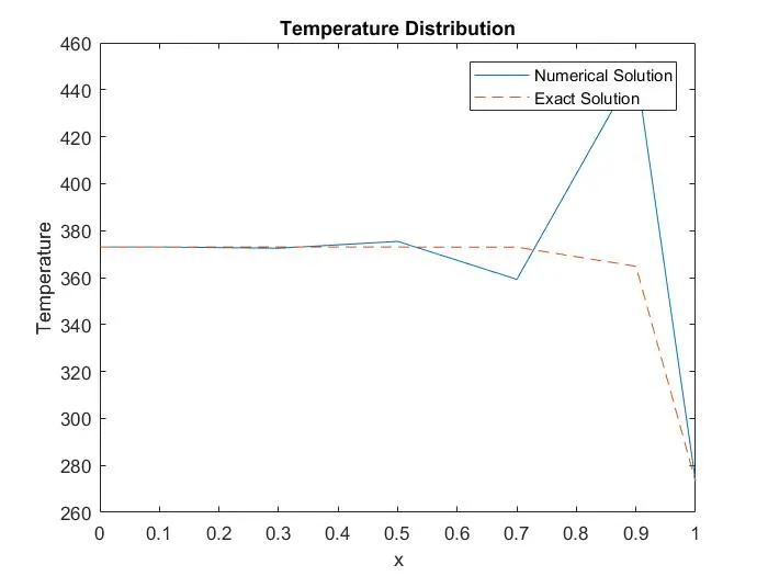

when n=10, u=2.5m/s


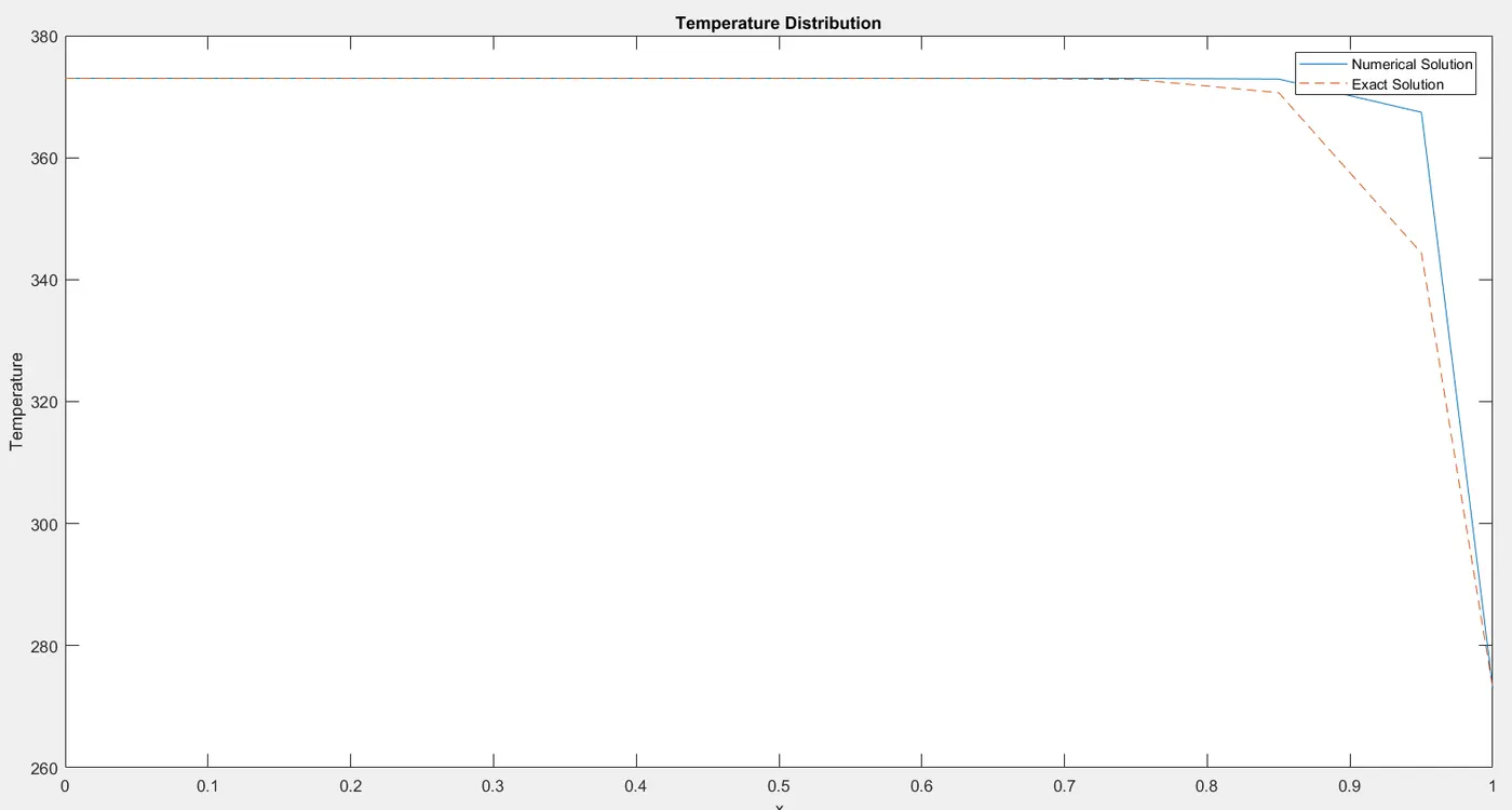
Assessment scheme:-
If the results of Hayase's and Leonard's QUICK result's are compared, it can be observed that accuracy of both the methods are the same i.e the solutions are equal to the extent of decimal values. This can be expected since equations used in both the methods are inherently the same one. But the one thing that is distinct between them is the solution with u=2.5 m/s and n=5. It is observed that due to the negative terms present in `a_P`for Leonard's method, the solution does not converge since `a_P`lost its dominancy at n=5 and u=2.5 m/s. But with Hayase's method, the system converged because the `a_P`in Hayase's method is that of Upwind method which cannot go negative and is always dominant and all the terms which could cause instability are put in delayed correction terms which obtains its values from previous iteration, ultimately helps the solution to converge. But the downside is that there are wiggles or upshoots observed in the scheme

Total Variation Diminishing Schemes
It is important to understand the aim behind developing these schemes. There are three objectives that these schemes drives to acheive:-
1)To maintain its accuracy similar to second order approximation schemes (QUICK)
2)To ensure convergence at all conditions and inputs of the system of equations.
3)To minimize wiggles and inputs as much as possible.

There is a path to developing these schemes which are needed to be followed to understand them.
i) The first is generalisation of upwind biased discretization schemes
It is to be understood that discretisation of diffusion terms is kept the same i.e central differencing scheme and this is to be carried forward. It is discretization of convective terms that require special attention. Lets first specify all the schemes and perform some special manipulation which may help in generalize them. Now for convenience schemes will be applied on east face and for u>0
a) Upwind Differencing(UD) scheme
`phi_e=phi_P` ...eq-1

b) Linear Upwind Differencing(LUD) scheme
This scheme is similar to upwind scheme but is of second order approximation.
`phi_e=phi_P+(phi_P-phi_W)/dx*dx/2`
It is basically exterpolation of curve ending at a nearest node upstream tangentially to get a value at the face of the cell.
It can be further simplified as
`phi_e=phi_P+(phi_P-phi_W)/2`
Now some special manipulation that has to be done is
`phi_e=phi_P+1/2(phi_P-phi_W)/(phi_E-phi_P)*(phi_E-phi_P)`...eq-2

c) QUICK scheme
`phi_e=phi_P+1/8[3phi_E-2phi_P-phi_W]`
Now some special manipulation, we get
`phi_e=phi_P+1/2[(3+(phi_P-phi_W)/(phi_E-phi_P))1/4]*(phi_E-phi_P)`..eq-3

d) Central differencing(CD) scheme
`phi_e=(phi_P+phi_E)/2`
Now after special manipualtion we get
`phi_e=phi_P+1/2(phi_E-phi_P)`...eq-4

Now observing equation 1,2,3 and 4, all the schemes can be generalized as

`phi_e=phi_P+1/2psi(phi_E-phi_P)`

where `psi=psi(r)` and `r=(phi_P-phi_W)/(phi_E-phi_P)`
So if `psi(r)=0`, the scheme is UD
if `psi(r)=1`, the scheme is CD
if `psi(r)=r`,the scheme is LUD
if `psi(r)=(3+r)/4`,the scheme is QUICK

Now Total Variation Diminishing scheme originates from studying `psi(r)`vs r graph. this graph is given by H K Versteeg and W Malalasekera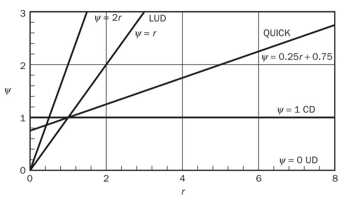


Now for a stable, non-oscilatory higher order scheme, the desirable property is monotonicity preserving.
A scheme is called monotonocity preserving if
i)it must not creat local extrema
ii)the value of an existing local minimum must be non-decreasing and that of a local maximum
must be non-increasing.
To understand TVD further consider this data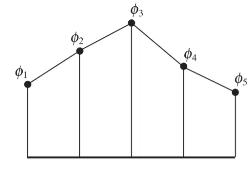


Total variation=`TV(phi)=abs(phi_2-phi_1)+abs(phi_3-phi_2)+abs(phi_4-phi_3)+abs(phi_4-phi_5)`
`TV(phi)=abs(phi_3-phi_1)+abs(phi_5-phi_3)`

So for monotonocity to be satisfied, total variation must not increase. Schemes in which total variation of discrete solution diminish with time are called Total Variation Diminishing or TVD. So a scheme is TVD if
`TV(phi_(n+1))<=TV(phi_(n))`
where n+1 and n are consecutive iterations.

Criteria for TVD scheme
Sweby(1984) gave necessary & sufficient conditions for a scheme to be TVD in terms of the `r-psi(r)` relationship
i)if 0<r<1, the upper limit is `psi(r)=2r`
ii)if `r>=1`, the upper limit is `psi(r)=2`
iii)if `r<=0`,`psi(r)=0`
The UD scheme is TVD
LUD scheme is not TVD for r>2
CD scheme is not TVD for r<0.5
QUICK scheme is not TVD for`r<3/7 & r>5`

So the idea of designing a TVD scheme is to introduce a modification in `psi(r)` so as to force the`r-psi(r)`relationship to remain within the shaded region for all possible values of r. This means in order to make the scheme TVD, we must constrain or limit the range of possible values of additional convective flux `Fe*psi(r)(phi_E-phi_P)/2` which was originally introduced to make UD scheme higher order.
Now since `psi(r)` adhering to make a scheme TVD limits overall convective flux to a specific operational area. `psi(r)` is called flux limiter function.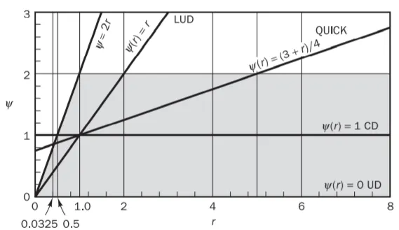


So for a scheme to be TVD, the flux limiter vs r or `psi(r)`vs r curve must liw in the shaded region.

Sweby(1984) also introduced the following requirement for 2nd order accuracy:-
1) the `(psi(r),r)` curve for the scheme must pass through (1,1) in `psi(r)` vs r graph for second-order accuracy.
2) if 0<r<1, lower limit is `psi(r)=r`, upper limit is `psi(r)=1`
if `r>=1,`lower limit is `psi(r)=1`, upper limit is `psi(r)=r`

Sweby introduced the symmetry property for limiter functions
`(psi(r))/r=psi(1/r)`
-this property ensures that backward & forward facing gradients are treated in the same facshion without need for special coding.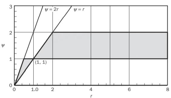

Now for a scheme to be TVD with second order accuracy, psi(r) vs r curve for the scheme must lie in the above shaded region and must pass through (1,1).

Now there various flux limiter functions which satisfy Sweby's requirements, they are as follows:-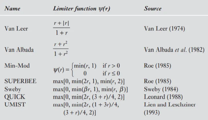


And the `psi(r)`vs r curve for each of the flux limiter functions are as shown with repect to the shaded area for sweby's conditions.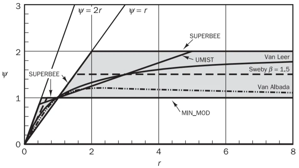

These images are taken from H K Versteeg and W Malalasekera
Now lets implement TVD scheme into a system of general equations for node.
Now we know that the numerical equation of governing equation,
`F_ephi_e-F_wphi_w=D_e(phi_E-phi_P)-D_w(phi_P-phi_W)`
So for a TVD scheme,
for u>0
`phi_e=phi_P+1/2psi(r_e^+)(phi_E-phi_P)`
`phi_w=phi_W+1/2psi(r_w^+)(phi_P-phi_W)`
for u<0
`phi_e=phi_E+1/2psi(r_e^-)(phi_P-phi_E)`
`phi_w=phi_P+1/2psi(r_w^-)(phi_W-phi_P)`

Basically r=upstream gradient/downstream gradient
So if u>0
`r_e^+=(phi_P-phi_W)/(phi_E-phi_P)` `r_w^+=(phi_W-phi_(WW))/(phi_P-phi_W)`
if u<0
`r_e^(-)=(phi_(E E)-phi_E)/(phi_E-phi_P)` `r_w^(-)=(phi_E-phi_P)/(phi_P-phi_W)`

Note:- - and + are notations to denote u>0 and u<0 respectively

So a general formula can be made for `r_e and r_w`

`r_e=(alpha_e*(phi_P-phi_W)+(1-alpha_e)*(phi_(E E)-phi_E))/(phi_E-phi_P)`

`r_w=(alpha_w*(phi_W-phi_(WW))+(1-alpha_w)*(phi_(E)-phi_P))/(phi_P-phi_W)`

where `alpha=1`if u>0 and `alpha=0`if u<0

Now these substitutions are made as they were done in previous scheme and transformed into a upwind scheme equation with a source term. The same general equation is border conditioned like in previous schemes and following generalized equation for all the nodes is found.
`a_(P_(UW))phi_P=a_(W_(UW))phi_W+a_(E_(UW))phi_E+Su_(UW)+bar (Su_e)+bar (Su_w)`.....`bar S`is segregated into `bar (Su_e) and bar (Su_w)`
`a_(P_(UW))=a_(W_(UW))+a_(E_(UW))+Sp_(UW)`



These system of equations were converted into a code and solved. There were certain discrepancies that were observed and mentioned in the book by H K Versteeg and W Malalasekera and some changes that are different from previous codes. These discrepancies are as follows:-

1)Now in the book it is said that DA=DB=D. But this substitution does not fit with the expression for upwind scheme which states that DA=DB=2*D. Now when this idea was put to test with the code. 2*D substitution gave a better fit than D. Hence DA=DB=2*D is used

2)Now it must be observed in Hayase and Leonard's QUICK scheme that the diffusion term at the face of the boundary node cell which is common with domain boundary is made consistent with the 2nd order approximation nature of the QUICK scheme. In the same way all the flux limiters that are displayed makes scheme of 2nd order accurate. This idea was tested in the code and it was found that curve was a better fit to the exact curve. Now we know that in quick scheme
`Gamma(dphi)/(dx)|_A=(DA)/3(9phi_P-8phiA-phi_E)` `Gamma(dphi)/(dx)|_B=(DB)/3(8phiB-9phi_P+phi_W)`.....DA=DB=D
but in the chapter it is considered,
`Gamma(dphi)/(dx)|_A=DA(phi_P-phiA)` `Gamma(dphi)/(dx)|_B=DB(phiB-phi_P)` DA=DB=2D
Now to make make one provided chapter to be consistent like in QUICK scheme, an extra correction term is added to the delayed source term for border nodes A and B.
So correction term for border node 1,
correction term`=D/3*(phi(i+1)-3*phi(i)+2*phiA)`
correction term for border node n,
correction term`=D/3*(2*phiB-3*phi(i)+phi(i-1))`

3)The system of equation fail to converge if Jacobi iterative method is applied for most of the flux limiter functions. It is found that when gauss seidel method is applied, only then the system converges. But it has to be kept in mind that gauss seidel is applicable to upwind terms as well as expressions present in Source terms. The gauss seidel application must be absolute to the equation.

4)Now for all the previous scheme, the initial output is taken as a constant zero or 1 at all points in the domain except the boundary values. But with TVD, since `r_e and r_w` have expressions such as`phi_P-phi_W or phi_E-phi_P` in the denominator, these expressions become zero at the first iteration and make `r_e and r_w` indeterminate. So its better to start with a initial value which is varying in any manner possible.
So the usual initial condition used is as follows

n=5;
L=1;%in meter
rho=1;%kg/m^3
T=0.1;
u=2.5;%m/s

%Derived Values

F=rho*u;
dx=L/n;
D=T/dx;
nx=n+2;% Position number
if u>=0
alpha=1;
else
alpha=0;
end
%Domain

x(1)=0;
x(2:nx-1)=(dx/2):dx:(L-(dx/2));
x(nx)=L;

%Initial Output

phiA=373;
phiB=273;
phi=zeros(1,nx);
phi(1)=phiA;
phi(nx)=phiB;

plot(x,phi)
xlabel('x')
ylabel('Temperature')
title('Temperature Distribution')

initial plot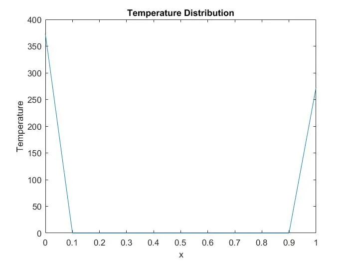


If this initial condition will be used, the system of equations will not converge for TVD scheme.

The correct initial condition is

n=5;
L=1;%in meter
rho=1;%kg/m^3
T=0.1;
u=2.5;%m/s

%Derived Values

F=rho*u;
dx=L/n;
D=T/dx;
nx=n+2;% Position number
if u>=0
alpha=1;
else
alpha=0;
end
%Domain

x(1)=0;
x(2:nx-1)=(dx/2):dx:(L-(dx/2));
x(nx)=L;

%Initial Output

phiA=373;
phiB=273;
phi=linspace(phiA,phiB,nx);

plot(x,phi)
xlabel('x')
ylabel('Temperature')
title('Temperature Distribution')

The plot for correct initial condition is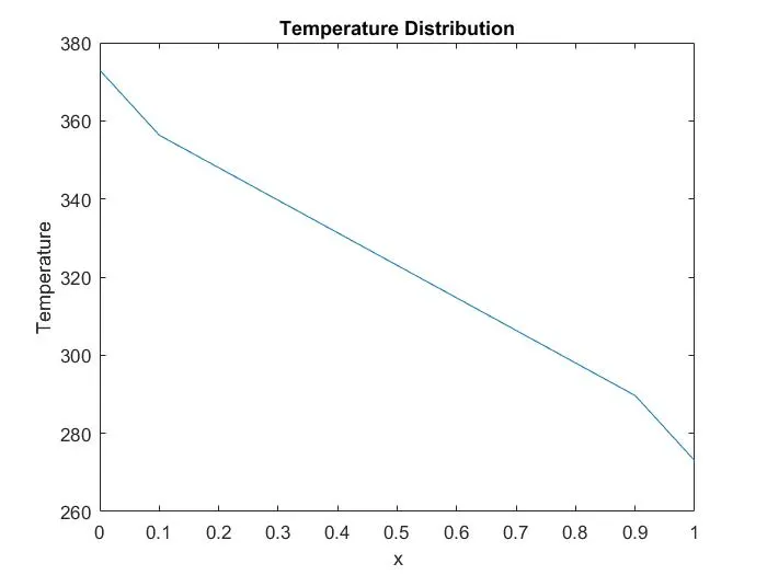


This is the correct initial condition. Various combinations can be tried but it will not make much difference.
Now before main code for the solver is displayed, a code was made prior to the main code for selection of flux limiter function or appropriate function depending on whether TVD scheme is selcted or a non-TVD scheme respectively. The code for the function is as follows:-

function [out]=Psi_function(r,beta,option)
%Appropriate Function

%Upwind Differencing Scheme
if option==1
out=0;
end
%Central Differencing Scheme
if option==2
out=1;
end
%Linear Upwind Differencing Scheme
if option==3
out=r;
end
%QUICK Scheme
if option==4
out=(3+r)/4;
end

%Flux Limiter Function

%Van Leer
if option==5
   if r>0
   out=(r+abs(r))/(1+r);
   else
   out=0;
   end
%out=2/(1+r);
end
% Van Albada
if option==6
   if r>0
   out=(r+r^2)/(1+r^2);
   else
   out=0;
   end
end
% Min-Mod
if option==7
   if r>0
   out=min([r 1]);
   else
   out=0;
   end
end
% SUPERBEE
if option==8
out=max([0 min([2*r 1]) min([r 2])]);
end
%Sweby
if option==9
out=max([0 min([beta*r 1]) min([r beta])]);
end
%QUICK
if option==10
out=max([0 min([2*r (3+r)/4 2])]);
end
%UMIST
if option==11
out=max([0 min([2*r (1+3*r)/4 (3+r)/4 2])]);
end
end

Now that the code for the function is displayed, the main code will be exhibited which will not only plot temperature distribution in the domain but will plot one more plot of `psi(r)`vs r plot in which a scatter plot of `r_e and r_w` with their respective `psi(r)`values will be shown. It is done to check whether the `psi and r`values that occur in the processing falls in the operating region specified by Sweby.
The main code is as follows

clear all
close all
clc
%Input

n=10;
L=1;%in meter
rho=1;%kg/m^3
T=0.1;
u=1;%m/s

%Derived Values

F=rho*u;
dx=L/n;
D=T/dx;
nx=n+2;% Position number
if u>=0
alpha=1;
else
alpha=0;
end
%Domain

x(1)=0;
x(2:nx-1)=(dx/2):dx:(L-(dx/2));
x(nx)=L;

%Initial Output

phiA=373;
phiB=273;
phi=linspace(phiA,phiB,nx);
phi(1)=phiA;
phi(nx)=phiB;


%Iteration Settings

tol=1e-5;
error=9e9;

% Appropriate function Psi
%Upwind Differencing Scheme----option==1
%Central Differencing Scheme----option==2
%Linear Upwind Differencing Scheme----option==3
%QUICK Scheme----option==4

% Flux Limiter Function
%Van Leer----option==5
%Van Albada----option==6
%Min-Mod----option==7
%SUPERBEE----option==8
%Sweby----option==9 beta=1.5
%QUICK flux limiter----option==10
%UMIST----option==11
option=5;
beta=1.5;
iter=0;
%Solver
while(error>tol)
phiold=phi;
iter=iter+1;
pos=0;
for i=2:nx-1
if i==2
   %Upwind Scheme Terms
   aw_uw=0;
   Aw=0;
   ae_uw=D-(1-alpha)*F;
   Ae=ae_uw*phiold(1,i+1);
   Sp_uw=2*D+F;
   Su_uw=Sp_uw*phiA;
   %Total Variation Diminishing terms
   rw=0;
   Psi_w=0;
   S_dc_w=0;
   re=(alpha*2*(phiold(1,i)-phiA)+(1-alpha)*(phiold(1,i+2)-phiold(1,i+1)))/(phiold(1,i+1)-phiold(1,i));
   Psi_e=Psi_function(re,beta,option);
   S_dc_e=((F/2)*((1-alpha)*Psi_e-alpha*Psi_e)*(phiold(1,i+1)-phiold(1,i)));
  cor_S=(D/3)*(phiold(i+1)-3*phiold(i)+2*phiA);
  %cor_S=0;
elseif i==3
   %Upwind Scheme Terms
   aw_uw=D+alpha*F;
   Aw=aw_uw*phi(1,i-1);
   ae_uw=D-(1-alpha)*F;
   Ae=ae_uw*phiold(1,i+1);
   Sp_uw=0;
   Su_uw=0;
   %Total Variation Diminishing terms
   rw=(alpha*2*(phi(1,i-1)-phiA)+(1-alpha)*(phiold(1,i+1)-phiold(1,i)))/(phiold(1,i)-phi(1,i-1));
   Psi_w=Psi_function(rw,beta,option);
   S_dc_w=(F/2)*(alpha*Psi_w-(1-alpha)*Psi_w)*(phiold(1,i)-phi(1,i-1));
   re=(alpha*(phiold(1,i)-phi(1,i-1))+(1-alpha)*(phiold(1,i+2)-phiold(1,i+1)))/(phiold(1,i+1)-phiold(1,i));
   Psi_e=Psi_function(re,beta,option);
   S_dc_e=(F/2)*((1-alpha)*Psi_e-alpha*Psi_e)*(phiold(1,i+1)-phiold(1,i));
   cor_S=0;
elseif i==nx-2
   %Upwind Scheme Terms
   aw_uw=D+alpha*F;
   Aw=aw_uw*phi(1,i-1);
   ae_uw=D-(1-alpha)*F;
   Ae=ae_uw*phiold(1,i+1);
   Sp_uw=0;
   Su_uw=0;
   %Total Variation Diminishing terms
   rw=(alpha*(phi(1,i-1)-phi(1,i-2))+(1-alpha)*(phiold(1,i+1)-phiold(1,i)))/(phiold(1,i)-phi(1,i-1));
   Psi_w=Psi_function(rw,beta,option);
   S_dc_w=(F/2)*(alpha*Psi_w-(1-alpha)*Psi_w)*(phiold(1,i)-phi(1,i-1));
   re=(alpha*(phiold(1,i)-phi(1,i-1))+(1-alpha)*2*(phiB-phiold(1,i+1)))/(phiold(1,i+1)-phiold(1,i));
   Psi_e=Psi_function(re,beta,option);
   S_dc_e=(F/2)*((1-alpha)*Psi_e-alpha*Psi_e)*(phiold(1,i+1)-phiold(1,i));
   cor_S=0;
elseif i==nx-1
   %Upwind Scheme Terms
   aw_uw=D+alpha*F;
   Aw=aw_uw*phi(1,i-1);
   ae_uw=0;
   Ae=0;
   Sp_uw=2*D-F;
   Su_uw=Sp_uw*phiB;
   %Total Variation Diminishing terms
   rw=(alpha*(phi(1,i-1)-phi(1,i-2))+(1-alpha)*2*(phiB-phiold(1,i)))/(phiold(1,i)-phi(1,i-1));
   Psi_w=Psi_function(rw,beta,option);
   S_dc_w=((F/2)*(alpha*Psi_w-(1-alpha)*Psi_w)*(phiold(1,i)-phi(1,i-1)));
   re=0;
   Psi_e=0;
   S_dc_e=0;
   cor_S=(D/3)*(2*phiB-3*phiold(1,i)+phi(1,i-1));
   %cor_S=0;
else
   %Upwind Scheme Terms
   aw_uw=D+alpha*F;
   Aw=aw_uw*phi(1,i-1);
   ae_uw=D-(1-alpha)*F;
   Ae=ae_uw*phiold(1,i+1);
   Sp_uw=0;
   Su_uw=0;
   %Total Variation Diminishing terms
   rw=(alpha*(phi(1,i-1)-phi(1,i-2))+(1-alpha)*(phiold(1,i+1)-phiold(1,i)))/(phiold(1,i)-phi(1,i-1));
   Psi_w=Psi_function(rw,beta,option);
   S_dc_w=(F/2)*(alpha*Psi_w-(1-alpha)*Psi_w)*(phiold(1,i)-phi(1,i-1));
   re=(alpha*(phiold(1,i)-phi(1,i-1))+(1-alpha)*(phiold(1,i+2)-phiold(1,i+1)))/(phiold(1,i+1)-phiold(1,i));
   Psi_e=Psi_function(re,beta,option);
   S_dc_e=(F/2)*((1-alpha)*Psi_e-alpha*Psi_e)*(phiold(1,i+1)-phiold(1,i));
   cor_S=0;
end
%Study start
pos=pos+1;
S_rw(iter,pos)=rw;
S_Psi_w(iter,pos)=Psi_w;
S_re(iter,pos)=re;
S_Psi_e(iter,pos)=Psi_e;
%study end
ap=aw_uw+ae_uw+Sp_uw;
S=S_dc_w+S_dc_e+Su_uw+cor_S;
phi(1,i)=(Aw+Ae+S)/ap;  
end
error=max(abs(phi-phiold));
end
max_r=max([max(max(S_rw)) max(max(S_re))]);
figure(1)
[phi_exact]=Exact_diffusion_Convection_Solver(rho,u,T,phiA,phiB,x);
plot(x,phi)
hold on
plot(x,phi_exact,'--')
xlabel('x')
ylabel('Temperature')
title('Temperature Distribution')
legend('Numerical Solution','Exact Solution')
hold off
figure(2)
plot([0 0.5],[0 1],'color','k');
hold on
plot([0 2],[0 2],'color','k');
hold on
plot([0.5 max_r+0.1],[1 1],'color','k');
hold on
plot([2 max_r+0.1],[2 2],'color','k');
hold on
for j=1:iter
plot(S_rw(j,1:pos),S_Psi_w(j,1:pos),'*','color','b');
hold on
plot(S_re(j,1:pos),S_Psi_e(j,1:pos),'*','color','b');
end
xlabel('r')
ylabel('psi(r)')
title('Verification of Sweby Condition')
legend('limits of the Swebys region')
axis([0 max_r+0.1 0 2.1]);

Now it was found that a lot can be done to study TVD itself but that goes out of the scope of the project.
Now Van leer flux limiter was selected with n=10 and u=1m/s.

The Temperature distribution plot is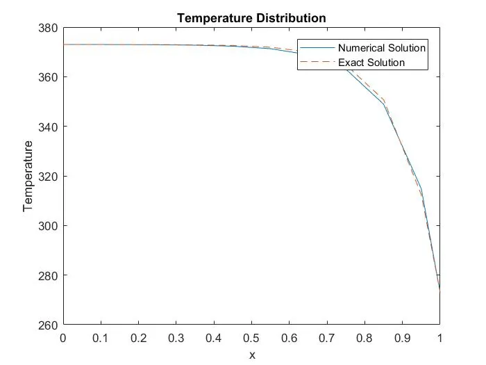


And the `psi(r)` vs r plot is as follows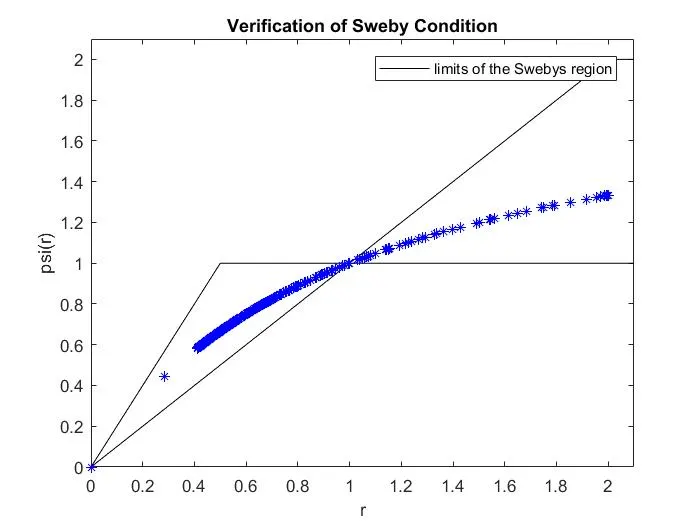


On observing the above graph, it can be found how the `(psi(r),r)`values for Van leer restrict themselves in Sweby's region

These plots will be compared for the same situation but using QUICK scheme by selecting option=4

For QUICK scheme,n=10 and u=1 m/s,
Temperature distribution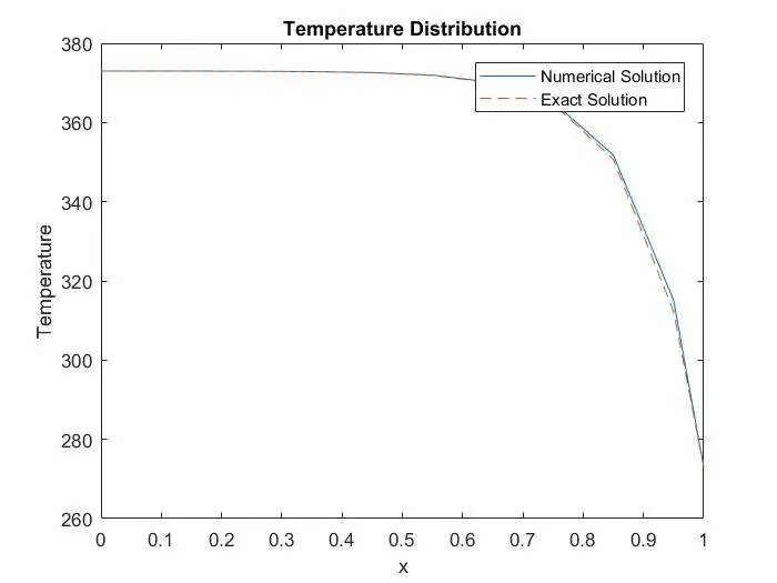


And the `psi(r)`vs r graph is as follows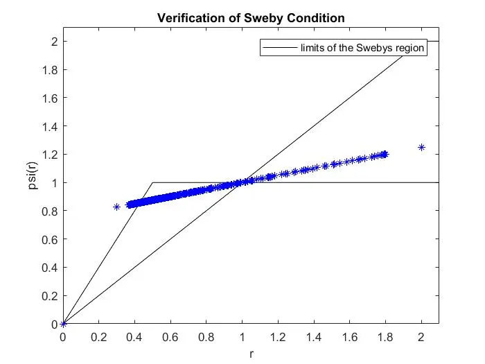

As it can be observed how `(psi(r),r)` points go beyond the region specified by Sweby which makes QUICK a non-TVD scheme.

Conclusion:-
Finite Volume method was studied from use of interpolation schemes to flux limiter functions. For each interpolation scheme, assessment was made in terms of its accuracy,stability and fluctuations in the solution. TVD scheme has much scope for study since various algorithms are employed with TVD to facilitate its purpose better. Some observations and formula derivations are of my own and extraneous to the material provided by H K Versteeg and W Malalasekera. Even TVD which is employed to control fluctuations which may occur for CD or QUICK schemes, it was found that they occur as well for TVD scheme when coupled with simple implicit iterative techniques. Various causes can be stipulated for this observation which is the scope for further research. Long step by step derivations were avoided to save time but ample explaination was given to facilitate understanding. All the observations were specified and all the findings explored.