Week 9 - FVM Literature Review
AIM:
- To describe the need for interpolation schemes and flux limiters in FVM.
Methods of Discretization:
- Finite Difference Method: Simple, straightforward to apply and Structured grid
- Finite Element Method: Applied to any geometry.
- Finite Volume Method: Conservative and Applied to any geometry.
Finite Volume Method:
The finite volume method (FVM) is a method for representing and evaluating partial differential equations in a of algebraic equations. In the FVM method, Volume integrals in the form of partial differential equation that contain divergence term converted in surface integrals, using the divergence theorem. These terms are then evaluated as fluxes at the surfaces of each finite volume. Because the flux entering a given volume is identical to that leaving to adjacent volume, these methods are conservative. Another advantage of FVM method is that it is easily formulated to allow for unstructured meshes. The method is used in many Computational Fluid Dynamics packages. ‘Finite Volume’ refers to small volume surrounding each node point on a mesh.
Steps in FV Discretization:
- Obtain the governing equation in integral form.
- Apply the Gauss Diversion Theorem
- Come up with suitable methods to calculate flux terms.
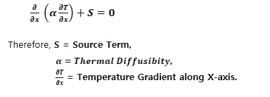
Consider 1D steady state heat conduction equation,
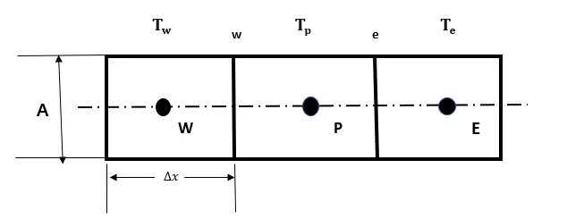
The governing equation is valid at every point in domain which means it is valid in entire control volume.
Multiplying governing equation by ‘dv’ and integrating it.
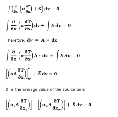
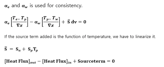
Alpha is kind of constant and not a function of temperature.
Types of Schemes:
- Gradient Scheme
- Interpolation Scheme
Gradient Scheme
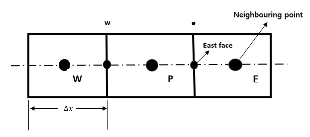
For calculating the temperature gradient at east face, we use neighbouring point temperature to numerically represent temperature gradient and this is referred as Gradient Scheme.
Interpolation Scheme
In Finite Volume Method, the solution is available only at the computational nodes. But we need to calculate the value of the variable that are not only present on the computational nodes, therefore we used interpolation technique to calculate the values of variable at non-computational nodes.
Types
- Upwind Interpolation
- Linear Interpolation
- Quadratic Upwind Interpolation
- Hybrid Interpolation
- Total Variation Diminish
Upwind Interpolation
It is used in numerical method in CFD for convection diffusion problem. This scheme is specific for Peclet number greater than 2 and less than -2.
The Upwind Interpolation scheme for approximation the value of a variable at the east face of control volume.
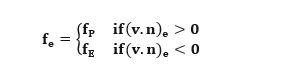
This interpolation scheme is equivalent to using backward or forward finite difference approximation. it is the first order accurate, and is numerically diffusive with a coefficient of numerical diffusion.
By taking into account the direction of flow, the upwind differencing scheme overcomes that inability of the central difference scheme. This scheme is developed for strong convection flows with suppressed diffusion effects.
Linear Interpolation
The liner interpolation is equivalent to use of central difference formula of the first order derivative and hence it is called as Central Difference Scheme.it is second order accurate whose accuracy is very good but we might have one small problem for advection dominated situations, that this scheme may produce oscillatory solutions. This scheme leads to simple approximation for evaluation of gradients required for evaluation of diffusion flux.
`f_e= f_E λ_e+ f_p (1-λ_e )`
`λ_e=(x_e-x_p)/(x_E-x_p )`
`λ_e` …….. Function which would depend on relative locations of the computational nodes E and P with respect to eastern face.
Quadratic Upwind Interpolation
The quadratic upwind interpolation is three order schemes, it is derived from the polynomial fitting. it is also represented as the QUICK interpolation on a uniform cartesian grid is given by,
`ϕ_e= 6/8 ϕ_(U ) + 3/8 ϕ_D - 1/8 ϕ_(UU)`
Where, D, U and UU donate the downstream, the first upstream and second upstream node respectively. Quick scheme is prone oscillation because of the third order.
Hybrid Interpolation
This scheme is combination of upwind interpolation scheme and central distribution scheme based on the local Peclet number.
`f_e= γf_(CDS)+(1-γ)f_(CDS)`
Total Variation Diminish
`f_e= f_p+ 0.5*ψ*r(f_e-f_p)`
`ψ = Local flux limiter r= Specified function which depends upon the local flow conditions
Flux Limiter:
Flux limiters are used in the numerical schemes to solve problem of fluid dynamics, described by highly coupled non-linear Partial Differential equations. If we tend to use low order numerical schemes for solving of the governing equations then we might get a highly oscillatory and unstable solution near discontinuity present. Whereas we tend to use higher order numerical schemes to capture the phenomenon more accurately we tend to exploit the power of computational unnecessarily. The main idea behind the use of flux limiters is to limit spatial derivative terms near the discontinuities to physical real values so as to maintain physical consistency. There are several types of flux/slope limiter functions. They came in handy when sharp wave-fronts/peaks are present. For smoothly changing wave/functions, the flux limiter does not operate and spatial derivative can be representing normally.
It is imperative note that flux limiter is also referred as slope limiters because they both have the same mathematical form, and both have effect of limiting the solution gradient near shocks and discontinuities.
`F(u_(i+1/2) )= f^(low) (i+1/2)- ϕ(r_i )(f^(low) (i+1/2)-f^(high) (i+1/2))`
`F(u_(i-1/2) )= f^(low) (i-1/2)- ϕ(r_i-1)(f^(low) (i-1/2)-f^(high) (i-1/2))`
Therefore,`f^(low)=Low Precision flux (Ist order Precise)`
`f^(high)=High Precision flux (Highest order Precise)`
`ϕ(r)=Flux limiter function and r= (u_(i )- u_(i-1 ))/(u_(i+1 )- u_(i ) )`