Week 9 - FVM Literature Review
Finite volume method:
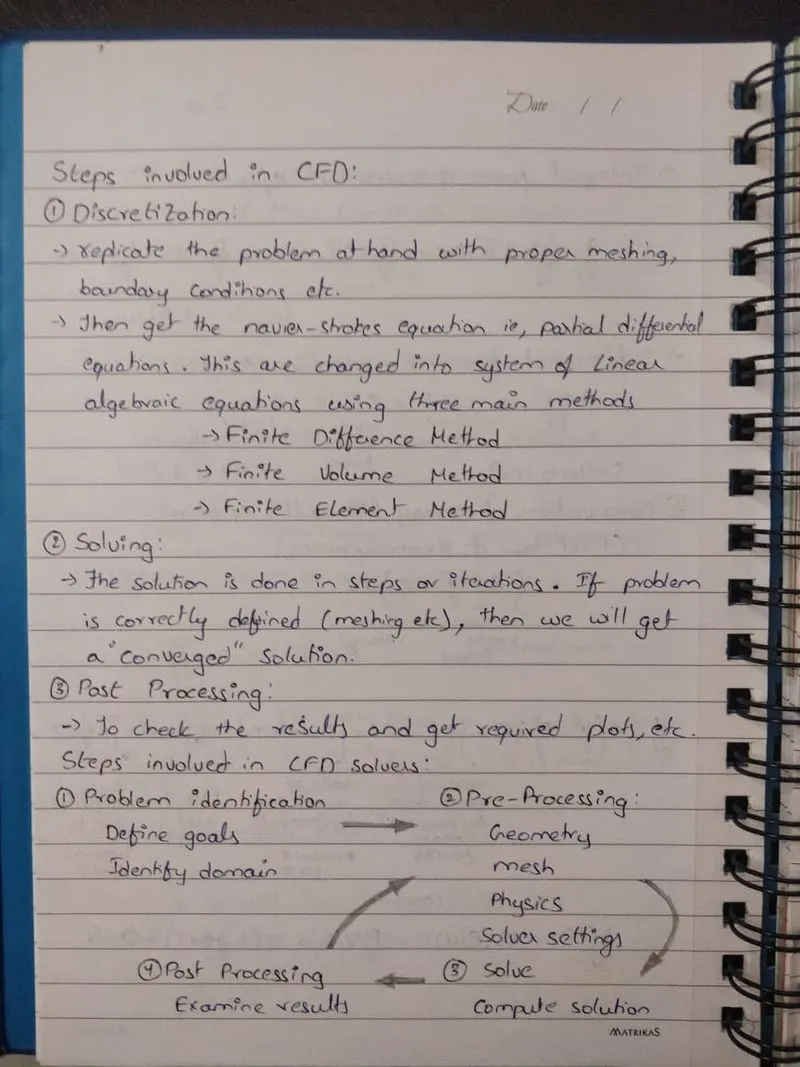
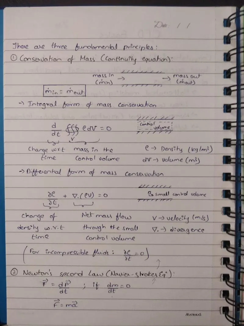
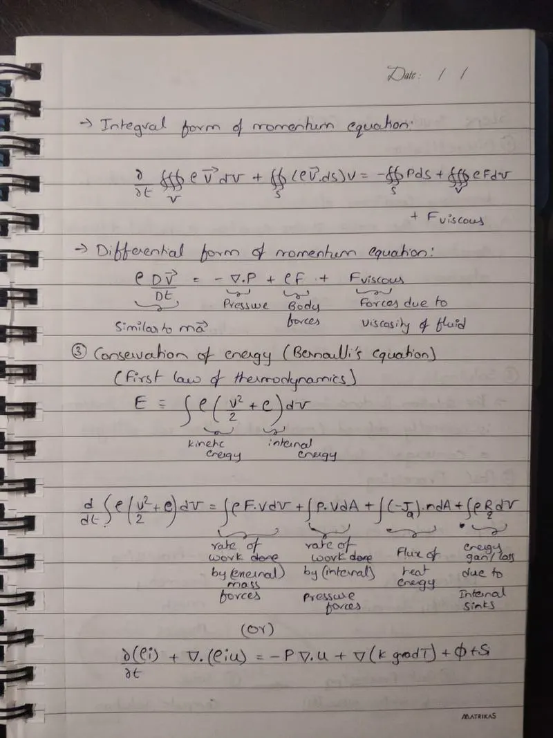
The finite volume method (FVM) is a method for representing and evaluating partial differential equations in the form of algebraic equations. In the finite volume method, volume integrals in a partial differential equation that contain a divergence term are converted to surface integrals, using the divergence theorem. These terms are then evaluated as fluxes at the surfaces of each finite volume. Because the flux entering a given volume is identical to that leaving the adjacent volume, these methods are conservative. Another advantage of the finite volume method is that it is easily formulated to allow for unstructured meshes. The method is used in many computational fluid dynamics packages. "Finite volume" refers to the small volume surrounding each node point on a mesh.
Differences between FDM & FVM:
Each method is quite similar in that it represents a systematic numerical method for solving PDEs. One important difference is the ease of implementation. A common opinion is that the finite-difference method is the easiest to implement and the finite-volume method the more difficult.
FDM:
The finite-difference method is defined dimension per dimension; this makes it easy to increase the “element order” to get higher-order accuracy. If you can fit the simulation in a rectangular or box-shaped geometry using a regular grid, efficient implementations are much easier than for finite-element and finite-volume methods. Regular grids are useful for very large-scale simulations on supercomputers often used in, as mentioned before, meteorological, seismological, and astrophysical simulations.
With the finite-difference method, you may easily run into problems handling curved boundaries for the purpose of defining the boundary conditions. Boundary conditions are needed to truncate the computational domain. They represent communication with the surrounding world, which is the part that you do not want included in your simulation. If one can overcome the boundary-condition problem on curved boundaries, the method gives very efficient and high quality results.
For computations that need high accuracy, the extra effort in making boundary-fitted meshes and the associated complications of such meshes for the implementation may be worth it. Examples include Formula 1 car computational-fluid-dynamic (CFD) simulations and space-shuttle CFD simulations. The finite-difference method is more difficult to use for handling material discontinuities. In addition, it does not lend itself for local grid refinement or anything similar to “adaptive mesh refinement.” This may be needed to resolve local rapid variations in solutions such as around a corner of a complex shape, as described earlier.
FVM:
The finite-volume method is a natural choice for CFD problems since the partial differential equations you have to solve for CFD are conservation laws. However, both finite differences and finite elements can also be used for CFD. Efficient technology for CFD with the finite-element method has become increasingly popular over the last 10 to 15 years. Techniques for CFD with the finite-difference and finite-volume method have been known and used much longer.
The finite-volume method’s strength is that it only needs to do flux evaluation for the cell boundaries. This also holds for nonlinear problems, which makes it extra powerful for robust handling of (nonlinear) conservation laws appearing in transport problems.
The local accuracy of the finite-volume method, such as close to a corner of interest, can be increased by refining the mesh around that corner, similar to the finite-element method. However, the functions that approximate the solution when using the finite-volume method cannot be easily made of higher-order. This is a disadvantage of the finite-volume method compared to the finite-element and finite-difference methods.
Need for interpolation schemes and flux limiters in FVM:
The approximation of surface and volume integrals may require values of the variable at locations other than the computational nodes of the CV. Values at these locations are obtained using interpolation formulae. This is why interpolation schemes are necessary for FVM.
Some of the interpolation schemes are:
- Upwind Interpolation Scheme(UDS)
- Central Differencing Approximation(CDS)
- Quadratic Upwind Differencing Scheme (QUICK)
- Total Variation Diminishing (TVD) Scheme
- Hybrid Interpolation Schemes(CDS and UDS)
For convective fluid flow, it is observed that the lower-order schemes are usually stable but quite dissipative in nature around the points of discontinuity or shocks while the higher-order schemes are unstable in nature and show oscillations in the vicinity of discontinuities or shocks. This is why flux limiters are used in FVM.
References:
https://en.wikipedia.org/wiki/Finite_volume_method
https://www.machinedesign.com/3d-printing-cad/fea-and-simulation/article/21832072/whats-the-difference-between-fem-fdm-and-fvm