Week 9 - FVM Literature Review

FINITE DIFFERENCE METHOD:

Finite difference methods is the numerical schemes used to solve partial differential equations. It consists in approximating the differential operator by replacing the derivatives in the equation using differential quotients. The domain is partitioned in space and in time and approximations of the solution are computed at the space or time points. The error between the numerical solution and the exact solution is determined by the error that is commited by going from a differential operator to a difference operator. This error is called the discretization error or truncation error. The term truncation error reflects the fact that a finite part of a Taylor series is used in the approximation.

Example: 1D unsteady state heat condution equation

`(delT)/(delt)=alpha(del^2T)/(delx^2)`

here grid spacing is well structure along coordinates.

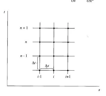
`(delT)/(delt)-alpha(del^2T)/(delx^2)=0`

Discretization of PDE:

select required approximation schemes(eg:central differencescheme)

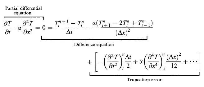
Avoid truncation error

Finally we obtain below equation:

`(T_i^(n+1)-T_i^(n))/(Deltat)=alpha(T_(i+1)^(n)-2T_i^(n)+T_(i-1)^(n))/(Deltax^2)`

Approaches:

Explict Method:

`T_i^(n+1)=T_i^(n)+alpha(Deltat)/(Deltax^2)(T_(i+1)^(n)-2T_i^(n)+T_(i-1)^(n))`

Implicit Method:

`(T_i^(n+1)-T_i^(n))/(Deltat)=alpha(1/2(T_(i+1)^(n+1)+T_(i+1)^(n))-1/2(2T_i^(n+1)+2T_i^(n))+1/2(T_(i-1)^(n+1)+T_(i-1)^(n)))/(Deltax^2)`

Demerits:

• FDM method is well suitable for well structured grid domains,because equations are write in every grid points.
• In unstructured grid domains, FDM method is quite complex,because this conditions are solved by Variable Transformation method where it has difficulty in coding.
• FDM is non conservative and discritized equations are not meaningful.
• So,FVM is used in unstructured grid domains

FINITE VOLUME METHOD:

The Finite volume method (FVM) is a widely used numerical technique.Based on the control volume formulation of analytical fluid dynamics, the first step in the FVM is to divide the domain into a number of control volumes ( cells, elements) where the variable of interest is located at the centroid of the control volume.

Furthermore, the FVM transforms the set of partial differential equations into a system of linear algebraic equations. Although the discrete approximation procedure in use in the FVM is distinctive, it also utilizes two basic steps. Firstly, it transforms and integrates the PDEs into balance equations over an element. The process incorporates the changing of the surface and volume integrals into discrete algebraic relations over elements as well as their surfaces using an integration quadrature of a specified order of accuracy.The resulting equation is called the discretized or discretization equation. In this manner, the discretization equation expresses the conservation principle for the variable inside the control volume.

Secondly, in this next step, the interpolation profiles are chosen to estimate the variation of the variables within the element and relate the surface values of the variables to their cell values and thus transform the algebraic relations into algebraic equations. In regards to the two steps in the FVM process, your approximation selection affects the overall accuracy of the subsequent numeric.

The most compelling feature of the FVM is that the resulting solution satisfies the conservation of quantities such as mass, momentum, energy, and species. This is exactlysatisfied for any control volume as well as for the whole computational domain and for any number of control volumes. Even a coarse grid solution exhibits exact integral balances.

FVM is the ideal method for computing discontinuous solutions arising in compressible flows. Any discontinuity must satisfy the Rankine-Hugoniot jump condition which is a consequence of conservation. Since finite volume methods are conservative they automatically satisfy the jump conditions and hence give physically correct weak solutions.

FVM is also preferred while solving partial differential equations containing discontinuous coefficients.

EXAMPLE: 1D steady state Heat Conduction equation

`rhoc_p(delT)/(delt)=del/(delx)(k(delT)/(delx))+del/(dely)(k(delT)/(dely))+del/(delz)(k(delT)/(delz))+S`

where "S" is source term

`alpha=k/(rhoc_p)`

for 1D and steady state,

`d/(dx)(alpha(dT)/(dx))+S=0`

convert differential form into integral form:

Integrate above equation in small elemental volume

`int_(dV)d/(dx)(alpha(dT)/(dx))dV+int_(dV)S dV=0`

• Grid generation:

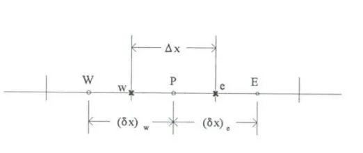
let `dV=Adx` and substitute in above eqn

`int_(dV)d/(dx)(alpha(dT)/(dx))Adx+int_(dV)S dV=0`

Derivation of Source Term(S):

Picard's Method:

The Picard’s iterative method gives a sequence of approximations y(t) to the solution of differential equations such that the nth approximation is obtained from one or more previous approximations.

This method of solving a differential equation approximately is one of successive approximation; that is, it is an iterative method in which the numerical results become more and more accurate, the more times it is used.

Apply taylor series

`S(t)=S(t_0)+((dS)/(dT))_(t_0)(T(t)-T(t_0))`

let

`S_u=S(t_0)-((dS)/(dT))_(t_0)T(t_0)`

`S_p=((dS)/(dT))_(t_0)`

`S(t)=S_u+S_pT_p`

let `S(t)=barSdV`

`barSdV=S_u+S_pT_p`

`int_(dV)d/(dx)(alpha(dT)/(dx))Adx+int_(dV)( S) dV=0`

for first term

limits of dv is from "w" to "e"

`int_(w)^ed/(dx)(alpha(dT)/(dx))Adx=int_(w)^ed(alpha(dT)/(dx))A`

`int_(w)^ed/(dx)(alpha(dT)/(dx))Adx=(alphaA(delT)/(delx))_w^e`

`(alphaA(delT)/(delx))_w^e=(alphaA(delT)/(delx))^e-(alphaA(delT)/(delx))^w`

`int_(w)^ed/(dx)(alpha(dT)/(dx))Adx=(alphaA(delT)/(delx))^e-(alphaA(delT)/(delx))^w`

`or above mesh generated condition,`alpha_eA_e((T_E-T_P)/(Deltax)_e)-alpha_wA_w((T_P-T_W)/(Deltax)_w)`

`int_(w)^ed/(dx)(alpha(dT)/(dx))Adx=alpha_eA_e((T_E-T_P)/(Deltax)_e)-alpha_wA_w((T_P-T_W)/(Deltax)_w)`

for second term

`int_(dV)S dV=barS DeltaV`

`int_(dV)S dV=(S_u+S_pT_p)`

where

`barS DeltaV=S_u+S_pT_p`

substitute derived first and second terms in above equation

`alpha_eA_e((T_E-T_P)/(Deltax)_e)-alpha_wA_w((T_P-T_W)/(Deltax)_w)+(S_u+S_pT_p) =0`

this equation seems as below:

[outlet heatflux]-[inlet heatflux]+[heat Source]=0

hence,

Even it is descritize,it seems to be meaningful terms.because it is conservative form.

• Discretization:

`alpha_eA_e((T_E-T_P)/(Deltax)_e)-alpha_wA_w((T_P-T_W)/(Deltax)_w)+(S_u+S_pT_p)`

`alpha_eA_e((T_P)/(Deltax)_e)+alpha_wA_w((T_P)/(Deltax)_w)-S_pT_P=alpha_eA_e((T_E)/(Deltax)_e)+alpha_wA_w((T_W)/(Deltax)_w)+S_u`

`((alpha_eA_e)/(Deltax)_e+(alpha_wA_w)/(Deltax)_w-S_p)T_P=((alpha_eA_e)/(Deltax)_e)T_E+((alpha_wA_w)/(Deltax)_w)T_W+S_u`

`a_pT_p=a_eT_e+a_wT_w+s_u`

where

`a_p=(alpha_eA_e)/(Deltax)_e+(alpha_wA_w)/(Deltax)_w-S_p`

`a_e=(alpha_eA_e)/(Deltax)_e`

`a_w=(alpha_wA_w)/(Deltax)_w`

• Setup the discretised equation at each of nodal points
• Modify the equation for the control volumes that are adjacent to the domain boundary
• Derive the system of linear algebraic equations
• Matrix solution techniques

INTERPOLATION SCHEMES:

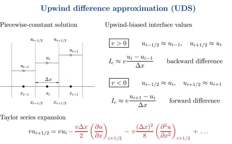
The approximation of surface and volume integrals may require valuesof the variables at locations other than the computational nodes of CV.Vales at this locations are obtained using interpolation schemes.

Upwind difference approximation (UDS):

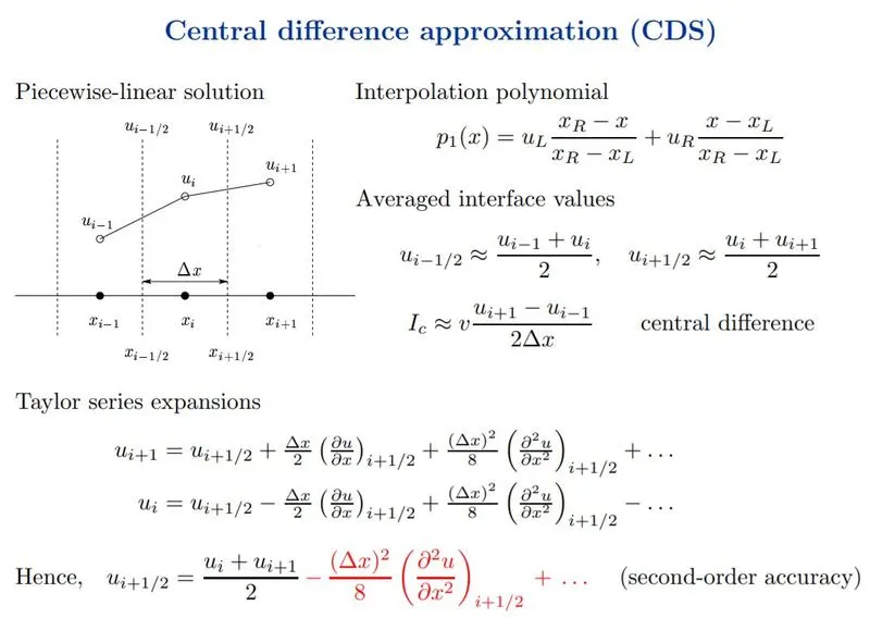
Central difference approximation (CDS):

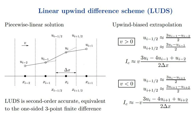
Linear upwind difference scheme (LUDS):

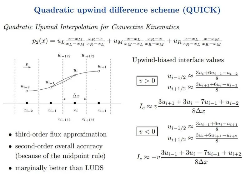
Quadratic upwind difference scheme (QUICK):

FLUX LIMITERS:

The behaviour of numerical schemes in order to capture shocks and discontinuity that arises in hyperbolic equations. Physically, these equations model the convective fluid flow. It has been observed that low-order schemes are usually stable but quite dissipative in nature around the points of discontinuity/shocks. On the other hand higher-order numerical schemes are unstable in nature and show oscillations in the vicinity of discontinuity. One can have a better understanding of such behaviour by analysing the modified equation of these schemes.

Now as said above one can not have high order accuracy without oscillations. The objective is to have highly accurate and stable oscillation free schemes. This kind of schemes are known as high resolution schemes. In 1984 Harten proposed the constuction and gave TVD(Total variation Diminishing)criteria for such scheme. Here we talk only about using flux limiters function to construct high resolution schemes. The idea is to tune the numerical flux of high order and low order scheme using the flux limiter function in such a way that the resulting scheme gives a high order accuracy in the smooth region of flow and sticks with first order of accuracy in the vicinity of socks/discontinuities .

The numerical flux fuction of high resolution conservative scheme as

`F_(j+1/2)=L_(j+1/2)+phi(theta)(H_(j+1/2)-L_(j+1/2))`

where

L,H are the numerical flux of conservative low order and high order schemes respectively.`phi` is a function of smoothness parameter `theta` usually defined as

`theta_j=(u_j-u_(j-1))/(u_(j+1)-u_j)`