Week 8 - Simulation of a backward facing step in OpenFOAM
Introduction:
In this study, We have a 2d block of length 0.20m and a height of 0.02m. We have an inlet of a height of 0.01. An incompressible viscous laminar flow is simulated using OpenFoam.
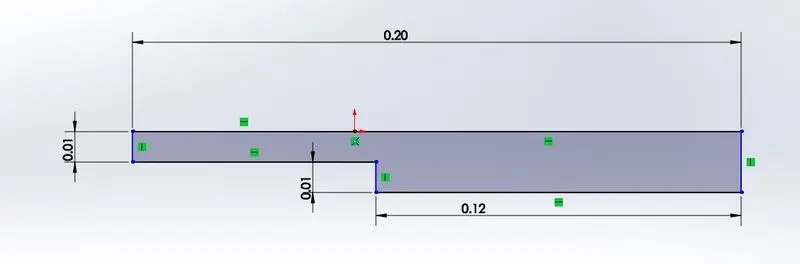
For the OpenFoam, We have to create geometry by dividing it into 5 blocks where vertices are stated.
In this, A flow is simulated through the backward-facing step. A study is being conducted at 0.085m from the inlet of the geometry and plots are drawn at the specified point.
Meshing: In this challenge, We have a mesh specification of 200 cells on the X-axis and 20 on the y-axis.
A grading factor is being used to decrease or increase the cell size near the walls. It helps to refine mesh more near the walls where we actually need results in simulation by compromising where we don't wanna look.
Objective:
In this study, we are going to,
- Simulate an incompressible laminar viscous flow through a backwards-facing step in OpenFoam.
- Case 1 - Simulate the flow without using any grading factor (i.e., GF = 1)
- Case 2 - Simulate the flow with a grading factor of 0.2. The cells should be finer near the walls (including the step wall).
Procedure:
- First, we have to find the solver in OpenFoam for incompressible laminar viscous flow. In this study, We are using an IcoFoam solver.
- The solver tutorial called cavity is being copied to the run folder and the boundaries are set according to specification.
- We have to define the geometry and Meshing in BlockMeshDict.
- After setting the start and end times in ControlDict, the initial conditions (i.e., pressure and velocity) are defined.
- The solver is run using the command icoFoam.
- Time taken for the simulation is being stated.
- The plots are drawn using ParaView.
Code for defining Geometry:
scale   0.1;

vertices
(
    (0 0 0)	        //0
    (8 0 0)   		//1
    (8 0.5 0)		//2
    (0 0.5 0)		//3
    (8 1 0)			//4
    (0 1 0)			//5
    (20 1 0)		//6
    (20 0.5 0) 		//7
    (20 0 0)		//8
    (20 -1 0)		//9
    (8 -1 0)		//10
    (0 0 0.1)		//11
    (8 0 0.1)		//12
    (8 0.5 0.1)		//13
    (0 0.5 0.1)		//14
    (8 1 0.1)		//15
    (0 1 0.1)		//16
    (20 1 0.1)		//17
    (20 0.5 0.1)	//18
    (20 0 0.1)		//19
    (20 -1 0.1)		//20
    (8 -1 0.1)		//21
);
Code for defining boundaries:
boundary
(
  inlet
    {
        type patch;
        faces
        (
            (0 11 14 3)
            (3 14 16 5)
        );
    }

    outlet
    {
        type patch;
        faces
        (
            (9 8 19 20)
            (8 7 18 19)
            (7 6 17 18)
        );
    }

    sidewalls
    {
        type wall;
        faces
        (
            (16 15 4 5)
            (15 17 6 4)
            (11 0 1 12)
            (10 21 12 1)
            (21 10 9 20)
        );
    }

    frontAndBack
    {
        type empty;
        faces
        (
            (0 3 2 1)
            (3 5 4 2)
            (10 1 8 9)
            (1 2 7 8)
            (2 4 6 7)
            (11 12 13 14)
            (13 15 16 14)
            (21 20 19 12)
            (12 19 18 13)
            (13 18 17 15)
        );
    }
);
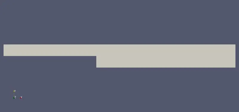
After defining the geometry, the following will be created in Paraview
For the initial conditions, we have a velocity of 0.66m/s
/*--------------------------------*- C++ -*----------------------------------*\
| =========                 |                                                 |
| \\      /  F ield         | OpenFOAM: The Open Source CFD Toolbox           |
|  \\    /   O peration     | Version:  v2012                                 |
|   \\  /    A nd           | Website:  www.openfoam.com                      |
|    \\/     M anipulation  |                                                 |
\*---------------------------------------------------------------------------*/
FoamFile
{
    version     2.0;
    format      ascii;
    class       volVectorField;
    object      U;
}
// * * * * * * * * * * * * * * * * * * * * * * * * * * * * * * * * * * * * * //

dimensions      [0 1 -1 0 0 0 0];

internalField   uniform (0 0 0);

boundaryField
{
     inlet
    {
        type            fixedValue;
        value           uniform (0.66 0 0);
    }

    outlet
    {
        type            zeroGradient;
    }

    sidewalls
    {
        type            noSlip;
    }

    frontAndBack
    {
        type            empty;
    }
}

// ************************************************************************* //
For the pressure, it is uniform and the code is as follows
/*--------------------------------*- C++ -*----------------------------------*\
| =========                 |                                                 |
| \\      /  F ield         | OpenFOAM: The Open Source CFD Toolbox           |
|  \\    /   O peration     | Version:  v2012                                 |
|   \\  /    A nd           | Website:  www.openfoam.com                      |
|    \\/     M anipulation  |                                                 |
\*---------------------------------------------------------------------------*/
FoamFile
{
    version     2.0;
    format      ascii;
    class       volScalarField;
    object      p;
}
// * * * * * * * * * * * * * * * * * * * * * * * * * * * * * * * * * * * * * //

dimensions      [0 2 -2 0 0 0 0];

internalField   uniform 0;

boundaryField
{
    movingWall
    {
        type            zeroGradient;
    }

    fixedWalls
    {
        type            zeroGradient;
    }

    frontAndBack
    {
        type            empty;
    }
}

// ************************************************************************* //
The start time for this problem is 0 sec and the end time is 3 seconds. These are values are given as inputs in ControlDict file in OpenFoam
The code in ControlDict is:
/*--------------------------------*- C++ -*----------------------------------*\
| =========                 |                                                 |
| \\      /  F ield         | OpenFOAM: The Open Source CFD Toolbox           |
|  \\    /   O peration     | Version:  v2012                                 |
|   \\  /    A nd           | Website:  www.openfoam.com                      |
|    \\/     M anipulation  |                                                 |
\*---------------------------------------------------------------------------*/
FoamFile
{
    version     2.0;
    format      ascii;
    class       dictionary;
    location    "system";
    object      controlDict;
}
// * * * * * * * * * * * * * * * * * * * * * * * * * * * * * * * * * * * * * //

application     icoFoam;

startFrom       startTime;

startTime       0;

stopAt          endTime;

endTime         3;

deltaT          0.001;

writeControl    timeStep;

writeInterval   20;

purgeWrite      0;

writeFormat     ascii;

writePrecision  6;

writeCompression off;

timeFormat      general;

timePrecision   6;

runTimeModifiable true;


// ************************************************************************* //
For the Grading factor, the given problem stated at the GradingFactor of 0.2
For the GF 0.2, the blocks for meshing is defined in the BlockMeshDict file as
blocks
(
    hex (0 1 2 3 11 12 13 14) (80 10 1) simpleGrading (0.2 0.2 1)
    hex (3 2 4 5 14 13 15 16) (80 10 1) simpleGrading (0.2 0.2 1)
    hex (10 9 8 1 21 20 19 12) (120 20 1) simpleGrading (5 5 1)
    hex (1 8 7 2 12 19 18 13) (120 10 1) simpleGrading (5 5 1)
    hex (2 7 6 4 13 18 17 15) (120 10 1) simpleGrading (5 0.2 1)
);
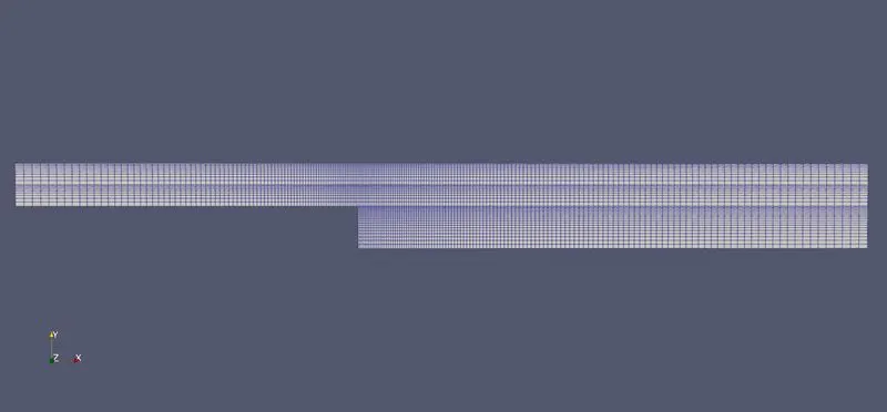
After solving the mesh will be followed:
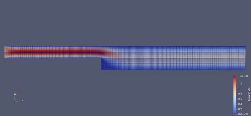
The simulation for velocity as follows:
Grading factor of 0.5:
code for the block:
blocks
(
    hex (0 1 2 3 11 12 13 14) (80 10 1) simpleGrading (0.5 0.5 1)
    hex (3 2 4 5 14 13 15 16) (80 10 1) simpleGrading (0.5 0.5 1)
	hex (2 7 6 4 13 18 17 15) (120 10 1) simpleGrading (2 0.5 1)
    hex (1 8 7 2 12 19 18 13) (120 10 1) simpleGrading (2 2 1)
	hex (10 9 8 1 21 20 19 12) (120 20 1) simpleGrading (2 2 1)
);
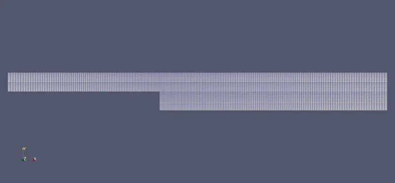
Mesh:
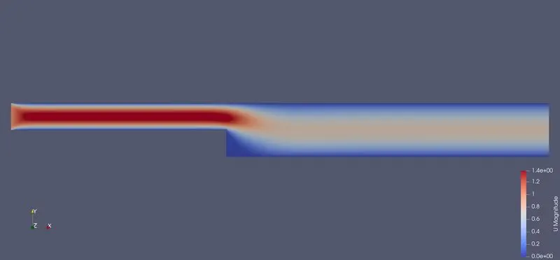
Simulation for velocity:
Grading factor of 1:
Code for the Block:
blocks
(
    hex (0 1 2 3 11 12 13 14) (80 10 1) simpleGrading (1 1 1)
    hex (3 2 4 5 14 13 15 16) (80 10 1) simpleGrading (1 1 1)
    hex (10 9 8 1 21 20 19 12) (120 20 1) simpleGrading (1 1 1)
    hex (1 8 7 2 12 19 18 13) (120 10 1) simpleGrading (1 1 1)
    hex (2 7 6 4 13 18 17 15) (120 10 1) simpleGrading (1 1 1)
);
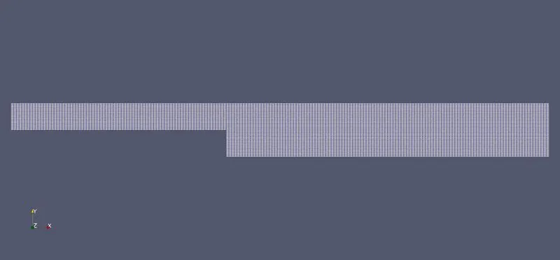
Mesh:
Simulation for velocity:
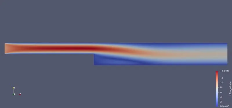
As we can see from the Meshes, The grading factor refines the mesh more near the walls. The simulation gets more detailed at the specific point where the mesh is refined more.
Comparison of Plots:
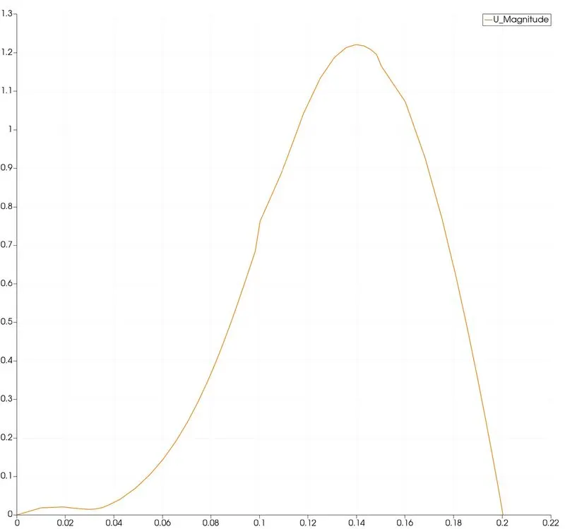
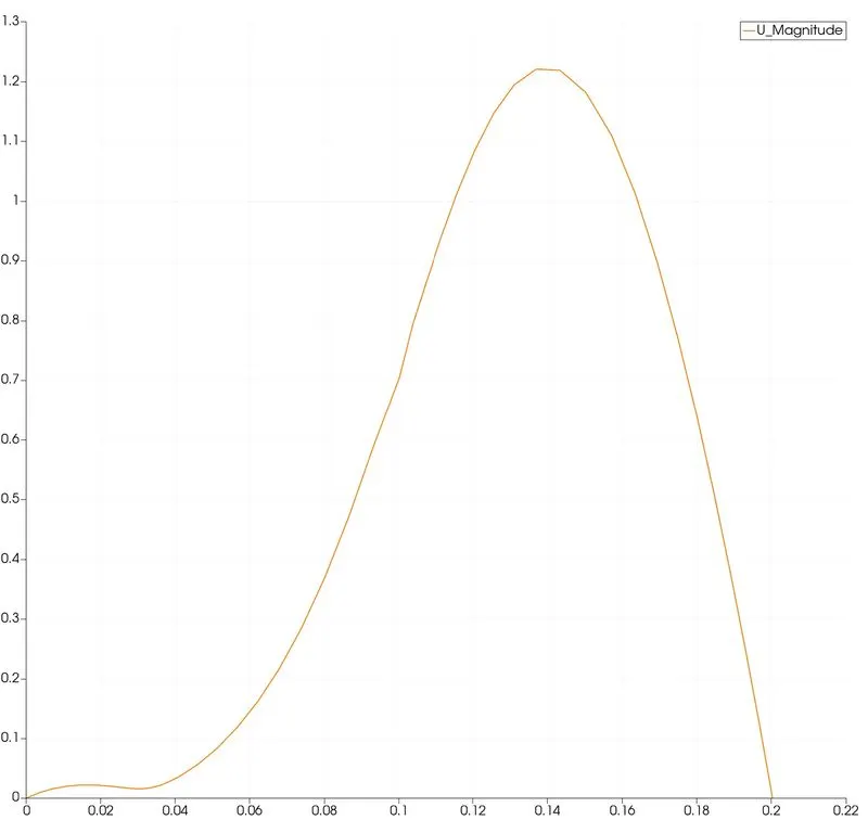
A plot over time is drawn at 0.085m from the inlet as the problem stated and we gonna compare at different grading factors.
Velocity plot over time for GF 0.2:
Velocity plot over time for GF 0.5:
Velocity plot over time for GF 1:
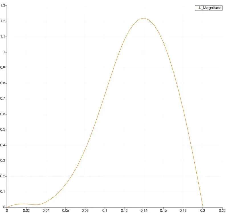
These plots are almost the same as the velocity peaks and drops as the area is increasing at the step, resulting in a decrease in velocity.
By comparing these plots, we could say the plot for GF 1 has a finer curve compared to GF 0.2 plot.
For GF 0.2 plot, there are sharp edges, as the mesh is not uniform and only finer near the walls, unlike the other 2 grading factors. Thus resulting in sharp edges unlike smooth curves in GF 1 and GF 0.5.
But there is a catch where the computational times and cost going to increase for GF 1 as the solver is trying to solve all the unnecessary regions compared to the specified region in GF 0.2.
And even more, the computational time in GF 0.2 is lower than the GF 1. So we have to choose the correct form for desired solution and cost.