Week - 8 Mass Scaling

G-drive:https://drive.google.com/drive/u/0/folders/1S18pT4BTUAOJ-_CcfmpdcvvKG5dY2Guq

AIM

• Adding the mass in and checking the run time and comparing the various mass scaling in the histogram graph

What is mass scaling

• Mass scaling enables an analysis to be performed economically without artificially increasing the loading rate. Mass scaling is the only option for reducing the solution time in simulations involving a rate-dependent material or rate-dependent damping, such as dashpots. In such simulations increasing the loading rate is not an option because material strain rates increase by the same factor as the loading rate. When the properties of the model change with the strain rate, artificially increasing the loading rate artificially changes the process.
• One of the methods used in the industry to reduce the run time of an explicit FEM analysis is a technique called “Mass scaling”.The run time of a FE simulation is mainly a function of the model size (the number of degrees of freedom) and the size of the solution step.

• As per the CFL (Courant-Friedrichs-Levy) condition, the stable time step for explicit analysis is

  

• Here e_min is the size of the smallest mesh element,c is the speed of the stress wave,The scaling factor is used for providing numerical stability,
• The smallest element in the mesh has the biggest impact on the run time.

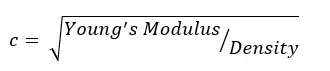
• Let’s see what ‘c’ is made of.

  

• where ρ">ρ is the material density.

  According to the above equations, artificially increasing the material density, ρ">ρ, by a factor of f2">f2f2 decreases the wave speed by a factor of f">ff and increases the stable time increment by a factor of f">ff. Remember that when the global stability limit is increased, fewer increments are required to perform the same analysis, which is the goal of mass scaling. Scaling the mass, however, has exactly the same influence on inertial effects as artificially increasing the loading rate. Therefore, excessive mass scaling, just like excessive loading rates, can lead to erroneous solutions. The suggested approach to determining an acceptable mass scaling factor, then, is similar to the approach to determining an acceptable loading rate scaling factor. The only difference to the approach is that the speedup associated with mass scaling is the square root of the mass scaling factor, whereas the speedup associated with loading rate scaling is proportional to the loading rate scaling factor. For example, a mass scaling factor of 100 corresponds exactly to a loading rate scaling factor of 10.

  There are several ways to implement mass scaling in your model using either fixed or variable mass scaling. The mass scaling definition can be changed from step to step, allowing great flexibility.

• If we increase the density of the smallest element (add mass actually!), the time step size increases which is what we want.

Defination of stabilty limit

• The stability limit is defined in terms of the highest frequency in the system (ωmax">ωmaxωmax). Without damping the stability limit is defined by the expression
• Δtstable=2ω/max, and with damping it is defined by the expression
• Δtstable=2ω/max(√1+ξ2−ξ),
• where ξ">ξξ is the fraction of critical damping in the mode with the highest frequency. (Recall that critical damping defines the limit between oscillatory and non-oscillatory motion in the context of free-damped vibration. Abaqus/Explicit always introduces a small amount of damping in the form of bulk viscosity to control high-frequency oscillations.) Perhaps contrary to engineering intuition, damping always reduces the stability limit.

The difference between using a positive or negative number for DT2MS in*CONTROL_TIMESTEP is as follows:

• Negative: Mass is added to only those elements whose timestep would otherwise be less than TSSF*abs(DT2MS). When mass scaling is appropriate, I recommend this method.

  Positive: Mass is added or taken away from elements so that the timestep of every element is the same. My opinion is there is no advantage to using this method over the negative DT2MS method and I find it harder to rationalize.

  The parameter MS1ST in *CONTROL_TIMESTEP controls whether mass is added only once during initialization (MS1ST=1) or anytime as necessary to maintain the desired timestep specified via DT2MS (MS1ST=0).

  You can use ENDMAS in *CONTROL_TERMINATION to stop the calculation aftera certain amount of mass has been added (active for automatic mass scaling only).

CASE STEUP TRIAL-1

• with out change of mass scaling dt2ms value is -3.5e-5 and the run time is 27hr 51min

Trial-2

• the dt2ms value is -4.5e-5 stil no added mass and the run time is 26hr8min

Trial-3

• the dt2ms value is -5.5e-5 the added mass is 2.855e3 and the run time is 23 hr15 min the run time is reduced and the percentage increase is 1.0034e-2

Trial-4

• the dt2ms value is -6.5e-5 the added mass is 1.6462e4 and the run time is 20 hr15 min the run time is reduced and the percentage increase is 5.7852e-2

Trial-5

• the dt2ms value is -7.5e-5 the added mass is 1.0608e5 and the run time is 16 hr36 min the run time is reduced and the percentage increase is 3.728e-1

Trial-6

• the dt2ms value is -8.5e-5 the added mass is 4.5162e5 and the run time is 13hr16 min the run time is reduced and the percentage increase is 1.5872e0

Trial-7

• the dt2ms value is -9.5e-5 the added mass is 1.2274e6 and the run time is 13hr38 min the run time is increase and the percentage increase is 4.3136

Trial-8

• the dt2ms value is -1.5e-4 the added mass is 3.2530e7 and the run time is 7hr51 min the run time is reduced and the percentage increase is 1.1432e2

Trial-9

• the dt2ms value is -1.1e-4 the added mass is 5.8027e6 and the run time is 10hr42 min the run time is increase and the percentage increase is 2.0393e1

Trial-10

• the dt2ms value is -1.05e-4 the added mass is 3.0583e6 and the run time is 10hr44 min the run time is increase and the percentage increase is 1.0748e1

Trial-11

• the dt2ms value is -1.02e-4 the added mass is 2.1276e6 and the run time is 10hr53min the run time is increase and the percentage increase is 7.4771

Trial-12

• the dt2ms value is -1.021e-4 and the added mass is 2.1438e6 as same as the runtime is 11hr 12min un time is increase the percentage increase is7.5342

Trial-13

• the dt2ms value is -1.022e-4 and the added mass is 2.1601e6 as same as the runtime is 11hr 12min un time is increase the percentage increase is7.5915

Trial-14

• the dt2ms value is -1.023e-4 and the added mass is 2.1766e6 as same as the runtime is 10hr 12min un time is the percentage increase is7.6493

Trial-15

• the dt2ms value is -1.024e-4 and the added mass is 2.1931e6 as same as the runtime is 11hr 00min un time is the percentage increase is7.7075

Trial-16

• the dt2ms value is -1.025e-4 and the added mass is 2.2098e6 as same as the runtime is 11hr 10min un time is the percentage increase is7.766

Trial-17

• the dt2ms value is -1.026e-4 and the added mass is 2.2350e6 as same as the runtime is 11hr 48min un time is the percentage increase is7.8548

Trial-18

• the dt2ms value is -1.275e-4and the added mass is 2.2520e6 as same as the runtime is 11hr 28min un time is the percentage increase is7.9145

Trial-19

• the dt2ms value is -1.028e-4and the added mass is 2.2692e6 as same as the runtime is 10hr 48min un time is the percentage increase is7.9747

Trial-20

• the dt2ms value is -1.029e-4and the added mass is 2.2761e6 as same as the runtime is 11hr 27min un time is the percentage increase is7.99

Trial-21

• the dt2ms value is -1.030e-4and the added mass is 2.279526 as same as the runtime is 11hr 16min un time is the percentage increase is8.066

After the 21 the objective is obtain 8.066

As same as implicit analysis

After adding the some importent impicit cards the run starts and obtain the normal termination

Histogram graph

Conculsion

• from this assignment we learn the what is mass scaling and how it use the run time
• we learn the how to add mass in materials
• what is differ between the implicit and explicit