Literature review - RANS derivation and analysis

Aim:-

• Write the original Governing Equation of Navier-strokes equations for the Boundary layer problem.
• Explain and apply Reynolds decomposition to the Navier-stroke equations.
• Perform Time Averaging on that equations.
• Explain the terms of the final Expression of Reynolds average Navier Strokes Equation.
• Also, Explain Turbulence viscosity and compare it with molecular viscosity

Governing Equations for the Boundary Layer:-

The following are the equation that governs the flow inside the boundary layer. These are nothing but Navier stokes equations that calculate the flow for boundary layer problems for any type of geometry. And we see for most of the cases we simulate the results for turbulence models. So, if we notice below three sets of equations, these equations are completely capable of giving us any type of flow either it is laminar or turbulent flows. Basically, if anyone implying this equation directly to solve fluid flow problem means they are using DNS (Direct Numerical Simulation) model. DNS is the technique of direct implementation of fluctuating values into the Navier-strokes equation without any turbulence model.

Continuity Equation

`(del u)/(del x) + (del v)/(del y) = 0`

Momentum Equation

`rho ((del u)/(del t) + (u del u)/(del x) + (v del u)/(del y)) = -(del P)/(del x) + mu (del ^2 u)/(del y^2)`

Energy Equation

`rho_c ((del T)/(del t) + (u del T)/(del x) + (v del T)/(del y)) = K(del^2 T)/(del x^2) + mu (del u)/(del y)^2`

Now, by using the above equations if we are fully capable of solving any fluid flow. Then why do we need a turbulence model?

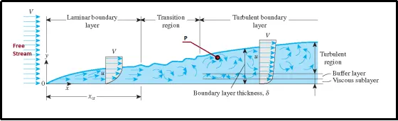
Let us understand the answer to the above question by an example. The above figure shows the boundary layer diagram where we have free stream velocity coming up from the left side on the stationary flat plate. The fluid actually flowing up over the stationary flat plate. Flow at the initial level is laminar and after some distance it becomes turbulent.

Now, if we put the velocity probe at the turbulent region, as portrayed in the figure by red dot labeled as point P. And if we measure the velocity in that point as the function of time, we well get fluctuating results of velocity as shown in below figure inside the red square.

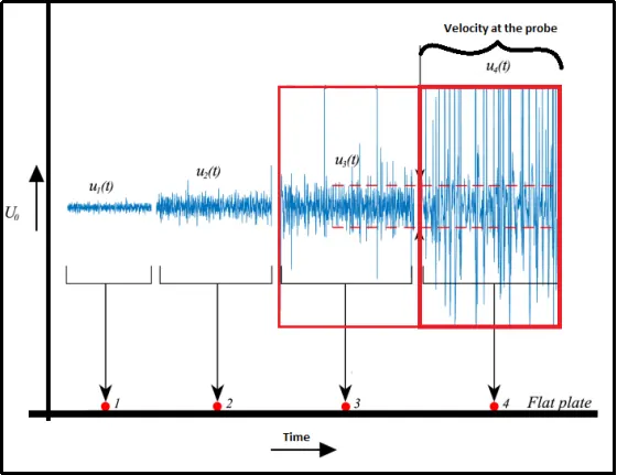
As we can see the velocity near the probe location will be continuously fluctuating for a very very small-time scale. Computing this problem for little time step with a huge number of computational cells requires an enormous amount of computation power and simulation may require endless time to complete. To overcome this problem we require turbulence models to simulate to capture the turbulence with coarser grids and larger time steps.

In the turbulence model, we are going to take this governing equation and integrating it with the much larger than the turbulent time step this is called the averaging process. Then we are going to apply something called Reynolds Decomposition and convert this original governing equation into a form called Reynolds Average Navier Stokes Equation.

Reynolds Decomposition

In this step, we are going to split our velocity or any other flow variable into a mean component and fluctuating component. this is called the Reynolds Decomposition.

`overbrace(u(x,y,z,t))^("Instantaneous velocity") = " "overbrace(bar u(x,y,z,))^("func. of Space") + overbrace(u’(x,y,z,t))^("func. of time and space")`

`" "v(x,y,z,t)" " =" " bar v(x,y,z,) +" " v’(x,y,z,t)`

`" "w(x,y,z,t)" "= " "ubrace(bar w(x,y,z,))_("Avg. quantity") + ubrace(w’(x,y,z,t))_("Time Avg. quantity")`

Mean Components:-

If we take a look at the following equation of `bar u` and `bar v` these are nothing but the time average. Here `bar u` and `bar v` are the function of only space with ineffective with change in change with time. which calculated for the time range 0 to `t_(i n t)`.

`bar u (x,y) = 1/(t_(i n t)) int_0^(t_(i n t)) u(x, y, t)dt`

`bar v (x,y) = 1/(t_(i n t)) int_0^(t_(i n t)) v(x, y, t)dt`

Fluctuating Components:-

If we integrate our fluctuating component, it is always going to be zero.

`1/(t_(i n t)) int_0^(t_(i n t)) u’(x, y, t)dt = 0`

To know 'why?' follow the below derivation.

`u(x,y,t) =bar u(x,y) + u’(x,y,t)`

`1/(t_(i n t)) int_0^(t_(i n t))u(x,y,t) = 1/(t_(i n t)) int_0^(t_(i n t))bar u(x,y) + 1/(t_(i n t)) int_0^(t_(i n t)) u’(x,y,t)`

`cancel(bar u(x,y) )= cancel(bar u(x,y)) + 1/(t_(i n t)) int_0^(t_(i n t)) u’(x,y,t)`

`1/(t_(i n t)) int_0^(t_(i n t)) u’(x,y,t) = 0`

Continuety Equation - Mass Conservation Equation

`(del u)/(del x) + (del v)/(del y) = 0`

After applying the Decomposition.

`(del(bar u+u'))/(del x) + (del(bar v+v'))/(del y) = 0`

Time Averaging of the above equation.

`1/(t_(i n t)) int_0^(t_(i n t)) [del/(del x) (bar u+u') dt + del/(del y) (bar v+v') dt ]=0`

Fluctuating Components will be zero. So, we will eliminate them.

`1/(t_(i n t)) int_0^(t_(i n t)) del/(del x) bar u dt + cancel(1/(t_(i n t)) int_0^(t_(i n t)) del/(del x) u' dt )+ 1/(t_(i n t)) int_0^(t_(i n t)) del/(del y) bar v dt + cancel(1/(t_(i n t)) int_0^(t_(i n t)) del/(del y) v' dt ) = 0`

Then We can write our equation as:

`(del bar u)/(del x) 1/(t_(i n t))int_0^(t_(i n t)) dt + (del bar v)/(del y) 1/(t_(i n t))int_0^(t_(i n t)) dt = 0`

After integrating with time we get:

`(del bar u)/(del x) [cancel((t_(i n t)-0))/cancel(t_(i n t))] + (del bar v)/(del y) [cancel((t_(i n t)-0))/cancel(t_(i n t))] =0`

In end result, we get our continuity equation as our time-averaged quantity.

`(del bar u)/(del x)+ (del bar v)/(del y) = 0`

Momentum Equation

The derivation of the time-averaged x-component of the momentum equation will be discussed now. The momentum equation for the x-component is given by:

`rho ((del u)/(del t) + (u del u)/(del x) + (v del u)/(del y)) = -(del P)/(del x) + mu (del ^2 u)/(del y^2)`

If we shift density term to the RHS, we get:-

`(del u)/(del t) + (u del u)/(del x) + (v del u)/(del y) = - 1/rho (del P)/(del x) + mu/rho (del ^2 u)/(del y^2)`

Then we will write `mu/rho` as kinematic viscosity `nu`

`(del u)/(del t) + (u del u)/(del x) + (v del u)/(del y) = - 1/rho (del P)/(del x) + nu (del ^2 u)/(del y^2)`

Then we are adding `[u((del u)/(del x)+(del v)/(del x))]` term as its output leads to zero value it is acceptable.

`(del u)/(del t) + (u del u)/(del x) + (v del u)/(del y) + [u((del u)/(del x)+(del v)/(del x))] = - 1/rho (del P)/(del x) + nu (del ^2 u)/(del y^2)`

Now, if we rearrange the equation, we get:-

`(del u)/(del t) + (del u del u)/(del x) + [(v del u)/(del y) + (u del v)/(del x)] = - 1/rho (del P)/(del x) + nu (del ^2 u)/(del y^2)`

We know that,

`del/(del y) (uv) = (v del u)/(del y) + (u del v)/(del x)`

So, we can put terms in our equation.

`(del u)/(del t) + (del u del u)/(del x) + del/(del y) (uv) = - 1/rho (del P)/(del x) + nu (del ^2 u)/(del y^2)`

Finally, we can write:

`(del u)/(del t) + (del u^2)/(del x) + (del(uv))/(del y) = - 1/rho (del P)/(del x) + nu (del ^2 u)/(del y^2)`

Adding Reynolds Decomposition

`1/(t_(i n t)) int_0^(t_(i n t)) {(del)/(del t)(bar u+u')dt + (del)/(del x) (bar u+u')^2 dt + (del)/(del y) [(bar u+u')(bar v +v')]}`

`= 1/(t_(i n t)) int_0^(t_(i n t)) [-1/rho (del (bar P + P’))/(del x) + nu (del^2)/(del y^2) (bar u + u’)dt]`

Now, we can eliminate fluctuating components from the equation.

`1/(t_(i n t)) int_0^(t_(i n t)) { (del bar u)/(del t) dt + cancel((del u')/(del t)dt) + (del bar u^2)/(del x) dt + (del u'^2)/(del x) dt + cancel((del bar u u')/(del x) dt )+ (del)/(del y) (bar u bar v) +cancel((del)/(del y) (bar u v'))+cancel((del)/(del y) (u' bar v)) + (del)/(del y) (u' v') }`

`=1/(t_(i n t)) int_0^(t_(i n t)) [ -1/rho (del bar P)/(del x) - cancel( 1/rho (del P’)/(del x))+ nu (del^2)/(del y^2) bar u dt + cancel( nu (del^2)/(del y^2) u’dt) ]`

After rearranging the above equation.

`(del bar u)/(del t) + (del bar u^2)/(del x) + (del)/(del y) (bar u bar v) = [ -1/rho (del bar P)/(del x) + nu (del^2)/(del y^2) bar u dt - 1/(t_(i n t)) int_0^(t_(i n t)) del /(del x) u’^2 dt - 1/(t_(i n t)) int_0^(t_(i n t)) (del)/(del y) (u' v') dt ]`

In general, the boundary layers are pretty thin if we compare them with the size of the plate. Therefore, the argument here can be made that the gradients of the velocity are going to be much stronger in the y-direction as compared to the x-direction. The changes in the gradients of the velocity made along the thickness of the boundary layer are huge and changes in the gradient of the velocity along the length of the plate are very little. Hence, we are going to neglect this term:-

`- 1/(t_(i n t)) int_0^(t_(i n t)) del /(del x) u’^2 dt`

After neglecting the above term we get our final term as:-

`underbrace((del bar u)/(del t) + (del (bar u)^2)/(del x) + (del(bar u bar v))/(del y) )_("Initial Terms")" "=``underbrace(-1/rho (del bar P)/(del x))_("Pressure Term")` `+``1/rho del/(del y) [underbrace(mu (del bar u)/(del y) dt)_("Viscous Stress term")``+``underbrace(rho/(t_(i n t)) int_0^(t_(i n t)) (del)/(del y) (u' v') dt)_("Reynolds Stress")]`

The derivation of the Reynolds-Averaged momentum equation is done. The boxed equations above are known as Reynolds-Averaged-Navier-Stokes equations (RANS).

The Above equation gives the expression for viscous stress and Reynolds stress.

Viscous Stress:-

• The viscous stresses are caused by the molecular diffusion across the boundary enclosing the control volume.
• If the molecular diffusion caused fluid molecules to move into a region of fluid with different velocities, then momentum is transferred and viscous stress exists.

Reynolds Stress:-

• Reynolds Stress results from the turbulent transport of momentum. The momentum flux is equivalently stress as it causes deformation of a fluid parcel.
• It is the component of the total stress tensor in a fluid obtained from the averaging operation over the Navier–Stokes equations to account for turbulent fluctuations in fluid momentum.

Turbulent Viscosity and its comparison with molecular viscosity:-

• Viscosity is the phenomenon (and the measure) of transverse momentum transport a moving fluid.
• In laminar flow, the mechanism of momentum transport is diffusion due to molecular motion and the resulting molecular collisions, the same as for mass transport and for heat conduction.
• In a turbulent flow, the mechanism of transverse momentum transport is dominated by bulk mixing at scales mostly well above the mean free path.
• So the effective viscosity in a region such as a turbulent boundary layer is much higher than in laminar flow.
• The more effective momentum transport due to the mixing in the turbulent boundary layer results in a thinner boundary layer between any wall in contact with the fluid and the free stream outside the boundary layer where the flow obeys potential flow laws.