Week 8: Literature review - RANS derivation and analysis
Apply reynold's decomposition to the NS equations and come up with the expression for reynold's stress.
- Explain your understanding of the terms reynold's stress
- What is turbulent viscosity? How is it different from molecular viscosity?
What is turnulence?
Turbulence is the state of chaotic and unstable fluid flow. First we take a brief look at the main characteristics of turbulent flows. The Reynolds number of a flow gives a measure of the relative importance of inertia forces (associated with convective effects) and viscous forces. In experiments on fluid systems it is observed that at values below the so-called critical Reynolds number Recrit the flow is smooth and adjacent layer of fluid slide past each other in an orderly fashion. If the applied boundary conditions do not change with time the flow is steady. This regime is called laminar flow.
At values of the Reynolds number above Recrit a complicated series of events takes place which eventually leads to a radical change of the flow character. In the final state the flow behaviour is random and chaotic. The motion becomes intrinsically unsteady even with constant imposed boundary conditions. The velocity and all other flow properties vary in a random and chaotic way. This regime is called turbulent flow. A typical point velocity measurement might exhibit the form shown in below Figure.
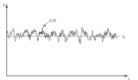
The random nature of a turbulent flow precludes an economical description of the motion of all the fluid particles. Instead the velocity in above Figure is decomposed into a steady mean value U with a fluctuating component u′(t) superimposed on it: u(t) = U + u′(t). This is called the Reynolds decomposition. A turbulent flow can now be characterised in terms of the mean values of flow properties (U, V, W, P etc.) and some statistical properties of their fluctuations (u′, v′, w′, p′ etc.).
How we characterizes the turbulence:
we characterizes the turbulence by using the reynolds numbers. The reynolds numbers quantify the turbulence level in a system. Basically it is the ratio of the inertial forces to viscous forces. The higher the Re, the more chaotic the turbulence. For a flow to be turbulent, Re must be much greater than the critical value. for example, Re for flow in a round pipe is
- Less than 2300 for laminar flow.
- Between 2300 and 4000 for transient flow.
- Greater than 4000 for turbulent flow.
Turbulence modeling approaches in Converge
Converge offers two modeling approaches
- Reynolds-Averged navier stokes equation (RANS)
- Large eddy simulation
Introduction
In spite of recent advances in scale-resolving CFD simulation capabilities, Reynoldsaveraged Navier-Stokes (RANS) methods are still widely used because of their lower expense and relative ease of use. However, RANS—which requires a turbulence closure model—is considered to be reliable only for attached flows. For flows with separation, some turbulence models fare better than others, and the level of variability and uncertainty generally increases with separation bubble size and flow complexity. For smoothbody separation bubbles in particular, most RANS models are known to underpredict the turbulence levels within the separated shear layer. As a result, reattachment and subsequent boundary layer recovery is typically delayed.
Turbulence modeling is an attempt to devise a number of partial differential equations for turbulent-flow calculation, based on appropriate approximations of the exact Navier–Stokes equations. In the approach of the Reynolds-averaged Navier–Stokes equations RANS the starting point is the Reynolds decomposition of the flow variables into mean and fluctuating parts, where the insertion of the Reynolds-decomposed variables into the Navier–Stokes equations—followed by an averaging of the equations themselves—gives rise to the Reynolds-stress tensor, an unknown term that has to be modeled in order for the RANS equations to be solved. The problem of the closure of the system of the Navier–Stokes equations essentially consists in this operation.
Historical background
Osborne Reynolds introduces the Reynolds decomposition and averaging of the Navier–Stokes equations. To arrive at their algebraic closure, the concept of eddy viscosity for the modeling of the Reynolds-stress tensor is then proposed. The first successful calculation of a practical turbulent flow is achieved in the 1920s by Prandtl , who introduced the concept of mixing length for the determination of the eddy viscosity. von Kármán, gave further contributions to the mixing-length approach that continues to be an active research field until the 1920s. By these times it becomes clear that the basic assumption behind the mixing-length approach—the direct analogy between the turbulent and the molecular-transport processes—is not realistic.
Transport equations for single-point moments of the velocity field was then started to be used to obtain modeled equations for the length and time scales of the velocity fluctuations, and Kolmogorov is probably the first to suggest the use of two distinct transport equations as a minimal set of expressions for turbulence modeling. Prandtl tied the eddy viscosity to the turbulent kinetic energy through the development of a separate transport equation, actually opening the way to the one-equation models, where the turbulence length scale is defined empirically and the turbulent kinetic energy is obtained from a specific transport equation. More widely used are the two-equation models and, in particular, the K−`epsilon` model where transport equations for the turbulent kinetic energy and the energy-dissipation rate are used. Almost all of the above turbulence closures rely on the concept of the eddy viscosity of and suffer from the drawbacks intrinsic to all the eddy-viscosity models, namely, the inability to properly account for streamline curvature, body forces, and history effects on the individual components of the Reynolds-stress tensor.
Rotta gave a fundamental contribution to a full Reynolds stress turbulence closure, actually succeeding in closing the Reynolds-stress transport equation and introducing the secondorder or second-moment models. The models based on the Reynolds-stress transport equation are usually able to account for history and nonlocal effects on the evolution of the components of
the Reynolds-stress tensor. In turn, because they require the solution of six additional transport equations for the individual components of the Reynolds-stress tensor, it has not been computationally feasible for the next few decades to solve complex engineering flows on the basis of full second-order closures. By the 1970s, with the initial availability of more powerful computers, the first works embodying second-order closure models start to appear. Launder developed a second-order closure model the Launder, Reece, and Rodi LRR model that significantly improves the work of Rotta. Systematic models for the pressure-strain correlation and the turbulent transport terms are derived and the modeled transport equation for the turbulent dissipation rate is solved in conjunction with the Reynolds-stress model.
Classification
Different classes of RANS turbulence models exist.
i) Zero-equation models. In this class, only a system of partial differential equations PDEs for the mean field is solved, and no other PDEs are used. These models are also called mean-velocity field MVF closures by Mellor and Herring.
ii) One-equation models. With respect to, this class involves an additional transport equation for the calculation of the turbulence velocity scale, usually cast in terms of
the average turbulent kinetic energy K.
iii) Two-equation models. With respect to ii, this class involves an additional transport equation for the calculation of the turbulence length scale, usually cast in terms of the
scalar dissipation rate of turbulent kinetic-energy. Classes ii and iii are also called mean turbulent energy MTE closures—representing a subset of the wider category of mean turbulent field MTF closures—by Mellor and Herring.
iv) Stress-equation models. With respect to i, this class involves a number of additional transport equations for the components of the Reynolds-stress tensor `tau_(ij)` and one for the scalar dissipation rate. For this reason, models of class iv are called `tau_(ij) - epsilon`models. These models are also called mean Reynolds-stress MRS closures by Mellor and Herring . They also represent a subset of the wider category of MTF closures, the latter including models of classes ii–iv.
Reynolda Averaged Navier Stokes equations
A turbulence model is defined as a set of equations (algebraic or differential) which determine the turbulent transport terms in the mean flow equations and thus close the system of equations. Turbulence models are based on hypotheses about the turbulent processes and require empirical input in the form of model constants or functions; they do not simulate the details of the turbulent motion, but only the effect of turbulence on the mean flow behavior. The concept of Reynolds averaging and the averaged conservation equations are some of the main concepts that form the basis of turbulence modeling.
The RANS are basically the Navier stokes equations that are time averaged after applying the Reynolds decomposition technique to the general NS equations. Solving the Navier stokes equations directly (Direct Numerical simulation) for a turbulent flow requires the grid to be very fine and that makes it impossible to solve these equations for engineering applications using even the supercomputers. On the other hand, DNS gives an extermely accurate results that is more than what is required by most engineering applications. Therefore this accuracy can be traded off to some extent to make the NS equations simpler to solve in an average computer for engineering applications. This is accomplished with the help of Reynold's averaging of the Navier-Stokes equations. This is accomplished with the help of Reynold's averaging of the Navier-Stokes equations.
Reynold's Decomposition
It is a mathematical technique that decomposes the flow variables of the Navier-Stokes equations into their mean and fluctuating components. This decomposition is necessary in order to be able to perform time-averaging of the entire Navier-Stokes equations.
According to Reynolds decomposition, the instantaneous velocity vector, u is defined as
`u = u^(bar) + u^(prime)`
Where
`u^(bar)` is the mean velocity
`u^(prime)` is the fluctuating velocity
In 3D flows
`u(x,y,z) = u^(bar)(x,y,z) + u^(prime)(x,y,z)` (1)
`v(x,y,z) = v^(bar)(x,y,z) + v^(prime)(x,y,z)` (2)
`w(x,y,z) = w^(bar)(x,y,z) + w^(prime)(x,y,z)` (3)
Depending upon the type of fluctuations (turbulence), there are three basic methods of determining the average value.
- Time averaging
- Spatial averaging
- Ensemble averaging
Time averaging
`u^(bar) = frac{1}t. int_0^t u(x,y,z)dt`
After integrating we get the average quantities and these average quantities does not change with time.
apply this average quantity on equation(1), we got
`frac{1}t. int_0^t u(x,y,z)dt = frac{1}t. int_0^t u^(bar)(x,y,z)dt + frac{1}t. int_0^t u^(prime)(x,y,z)dt`
Where, `u^(bar)` is not a function of time. hence, when we integrate fluctuating component it's always be zero.
`frac{1}{t} .int_0^(t) u^(prime)(x,y,z,t) dt = 0`
Therefore, when we integrate fluctuating terms for longer time period this term would be zero.
Continuity equation
`frac{du}{dx} = 0`
substitute, `u = u^(bar) + u^(prime)`
`frac{d(u^(bar)+u^(prime))}{dx} =0`
Take time average of whole equation.
`frac{1}t. int_0^t [frac{d}{dx}(u^(bar)+u^(prime))dt] =0`
`frac{1}t. int_0^t frac{d}{dx}(u^(bar))dt + frac{1}t. int_0^tfrac{d}{dx}(u^(prime))dt =0`
Since, time integrating of fluctuating component is zero and also, integral limits is not a function of x.
`frac{du^(bar)}{dx}frac{1}t int_0^t dt =0`
`frac{d(u^(bar))}{dx}frac{(t-0)}{t) =0`
`frac{d(u^(bar))}{dx}fr =0`
`frac{d(u^(prime))}{dx}fr =0`
Time averaged flow field and unsteady velocity fluctuations field obeys continuity.
Conservation of momentum:
Conservation from of N-S equation is,
`rho. (frac{du}{dt}+ufrac{du}{dt}+vfrac{du}{dt)) = -frac{dP}{dx}+ mu. frac{d^2u}{dy^2}`
where, `nu = frac{mu}{rho}`
Equation will be rewrite as,
`(frac{du}{dt}+ufrac{du}{dt}+vfrac{du}{dt)) = -(frac{1}{rho})frac{dP}{dx}+ nu. frac{d^2u}{dy^2}`
from product rule,
`frac{d}{dy}(u.v) = ufrac{dv}{dy} + vfrac{du}{dy}`
`frac{du}{dt} + 2u.frac{du}{dx} +frac{d}{dy}(u.v) = -(frac{1}[rho}) frac{dP}{dx}+nu. frac{d^2u}{dy^2}`
`frac{du}{dt} + frac{du^2}{dx} +frac{d}{dy}(u.v) = -(frac{1}[rho}) frac{dP}{dx}+nu. frac{d^2u}{dy^2}`
Put, `u = u^(bar)+u^(prime)` & `v = v^(bar)+v^(prime)`
Applying Reynold's decomposition
`frac{1}{t} int_0^t [frac{d(u^(bar) +u^prime)}{dt} + frac{d(u^(bar) +u^prime)^2}{dt} +frac{d}{dy}((u^(bar)+u^(prime)).((v^(bar)+v^(prime))].dt = frac{1}{t} int_0^t [-(frac{1}{rho})frac{d(P^(bar) +P^prime)}{dx}].dt + nu frac{d^2}{ dy^2}{(u^(bar) +u^prime)}{dt}`
Since the time averaged of flucatuation term is zero. Equation reduced to
`frac{du}{dt} + frac{d(u^(bar))^2}{dx} +frac{d(u^(prime))^2}{dx}+frac{d(u^(bar).v^(bar))}{dy}+frac{d(u^(prime).v^(prime))}{dy} = -(frac{1}{rho}) frac{dP^bar){dx} +nu. frac{d^2u^(bar)}{dy^2}`
`frac{du}{dt} +frac{d(u^(bar))^2}{dx}+frac{d(u^(bar).v^(bar))}{dy} = -(frac{1}{rho}) frac{dP^bar){dx} +nu. frac{d^2u^(bar)}{dy^2}- frac{d(u^(prime))^2}{dx}- frac{d(u^(prime).v^(prime))}{dy}`
We can write above equation as,
`frac{du}{dt} +frac{d(u^(bar))^2}{dx}+frac{d(u^(bar).v^(bar))}{dy} = -(frac{1}{rho}) frac{dP^bar){dx} +nu. frac{d^2u^(bar)}{dy^2}- frac{1}{t} int_0^t frac{d(u^(prime))^2}{dx}- frac{1}{t} int_0^tfrac{d(u^(prime).v^(prime))}{dy}dt`
Assume changes along X-direction is negligible compare to changes along Y-direction inside Boundary layer, Hence
`frac{1}{t} int_0^t frac{d(u^(bar))^2}{dx}.dt =0`
Equation becomes
`frac{du}{dt} +frac{d(u^(bar))^2}{dx}+frac{d(u^(bar).v^(bar))}{dy} = -(frac{1}{rho}) frac{dP^bar){dx} +nu. frac{d^2u^(bar)}{dy^2}- frac{1}{t} int_0^tfrac{d(u^(prime).v^(prime))}{dy}dt`
Considering RHS of above equation:
RHS = `-(frac{1}{rho}) frac{dP^bar){dx} +nu. frac{d^2u^(bar)}{dy^2}- frac{1}{t} int_0^tfrac{d(u^(prime).v^(prime))}{dy}dt`
`-(frac{1}{rho}) frac{dP^bar){dx} + frac{1}{rho}.frac{d}{dy}[mu. frac{du^(bar)}{dy}- frac{rho}{t} int_0^t (u^(prime ).v^(prime)).dt]`
(frac{1}{rho}) frac{dP^bar){dx} Pressure Term
`u. frac{du^(bar)}{dy}` Molecular Viscosity
`frac{rho}{t} int_0^t (u^(prime ).v^(prime)).dt` Momentum Diffusivity
Reynolds Stress
The Reynolds stress is a mechanism for generation of sheared flow from turbulence.The momentum flux is equivalently a stress as it causes deformation of a fluid parcel. It is not because of the existence of a real tangential force (as in viscous stress). Reynolds stress is a property of the flow. It is a result from turbulent transport of momentum. The momentum flux is equivalently a stress as it causes deformation of fluid parcels. It is not because of existence of real tangential force (as in viscous stress). It is property of flow.
We consider a homogeneous fluid, whose density `rho`is taken to be a constant. For such a fluid, the components of `tau_(ij)^(prime) = -rho (u^(prime) . v^(prime))^(bar)`
where `(u^(prime) . v^(prime))^(bar)`is average advection of u and v.
Advection of momentum or veocity fluctuation results in a spread of momentum by turbulence. This term describes the diffusive nature of turbulence. The negative divergence of the Reynolds stresses represents convective momentum transfer due to the random motion of macroscopic fluid packets(eddies)
Thus, a non-zero value of the gradient of the Reynolds stress (of fluctuating flow components) can drive a laminar flow.
Stress term from the Reynolds average of the
Stress term from the Reynolds average of the
`tau_(R_(xz) = tau_(R_(zx) = -rho (u^(prime)w^(prime))^(bar)``
`tau_(R_(yz) = tau_(R_(zy) = -rho (v^(prime)w^(prime))^(bar)``
`tau_(R_(xy) = tau_(R_(yx) = -rho (u^(prime)v^(prime))^(bar)``
To describe reynold stress tensor:
`[[(u^(prime) u^(prime))^(bar), (u^(prime) v^(prime))^(bar), (u^(prime) w^(prime))^(bar)], [(v^(prime) u^(prime))^(bar), (v^(prime) v^(prime))^(bar), (v^(prime) w^(prime))^(bar)],[(w^(prime) u^(prime))^(bar), (w^(prime) v^(prime))^(bar), (w^(prime) w^(prime))^(bar)]]`
A second order tensor which is symmetric matrix.
- What is turbulent viscosity? How is it different from molecular viscosity?
Viscosity is the phenomenon (and the measure) of transverse momentum transport a moving fluid. In laminar flow the mechanism of momentum transport is diffusion due to molecular motion and the resutlting molecular collisions, the same as for mass transport and for heat conduction. In a turbulent flow, the mechanism of transverse momentum transport is dominated by bulk mixing at scales mostly well above the mean free path. So the effective viscosity in a region such as a turbulent boundary layer is much higher than in laminar flow. The more effective momentum transport due to the mixing in the turbulent boundary layer results in a thinner boundary layer between any wall in contact with the fluid and the free stream outside the boundary layer where the flow obeys potential flow laws.
The coefficients that relates the average shear stress and rate of velocity gradient in the turbulent flow is called turbulent viscosity. The viscosity in turbulence is non-homogeneous and it varies in space.
The relation between turbulent stress `tau_(turb)` and turbulent viscosity `mu_t`is
`tau_(turb) = -rho. (u^(prime) v^(prime))^(bar)`
`tau_(turb) = mu_t frac{du}{dy}`
Turbulent viscosity is the turbulent transfer of momentum by eddies give rise to internal fluid friction which is analogous to the action of molecular viscosity in laminar flow but takes place in much larger space.
Molecular viscosity is the same as viscosity. The coefficients of molecular viscosity the same as the dynamic viscosity. Molecular viscosity is the transport of mass motion momentum solely by the random motions of individual molecules not moving togetherin coherent groups.
In general the shear stress may be written as
`tau = tau_(laminar)+tau_(turb)`
`tau = mu frac{du}{dy} + (-rho.(u^(prime)v^(prime))^(bar))`
The first term in the above equation is the result of viscous effects and second term is the result of turbulent effect. If flow is laminar then the fluctuation terms are zero.