Week 8: Literature review - RANS derivation and analysis

#Intention: 1.To apply Reynold's decomposition to Navier stokes equations .

                   2.Derive an expression for Reynold's stress.

#Need of Reynold's Decomposition:

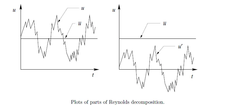
In fluid dynamics and turbulence theory, Reynolds decomposition is a mathematical technique used to separate the expectation value of a quantity from its fluctuations. For example, for a quantity 'u'  the decomposition would be

 

where  denotes the expectation value of , (often called the steady component/time, spatial or ensemble average), and , are the deviations from the expectation value (or fluctuations). The fluctuations are defined as the expectation value subtracted from quantity } such that their time average equals zero

The expected value, , is often found from an ensemble average which is an average taken over multiple experiments under identical conditions. The expected value is also sometime denoted , but it is also seen often with the over-bar notation

Direct Numerical Simulation, or resolving the Navier-Stokes equations completely in `(x,y,z,t)`, is only possible on small computational grids and small time steps when Reynolds numbers are low. Due to computational constraints, simplifications of the Navier-Stokes equations are useful to parameterize turbulence that are smaller than the computational grid, allowing larger computational domains.

Reynolds decomposition allows the simplification the Navier–Stokes equations by substituting in the sum of the steady component and perturbations to the velocity profile and taking the mean value. The resulting equation contains a nonlinear term known as the Reynolds stresses which gives rise to turbulence.

-------------------------------------------********************---------------------------------------------

Governing Equations for Boundary layer:

`(delu)/(delx)+(delv)/(dely)=0`---------------Continuity Equation----------------------------(1)

`rho((delu)/(delt)+u(delu)/(delx)+v(delu)/(dely))=-(delP)/(delx)+mu(del^2u)/(dely^2)`-----------Momentum Equation----------------(2)

Reynold's Decomposition:

Instantaneous Velocity= Time average velocity + Fluctuating component of Velocity

u= Instantaneous Velocity

`u^-`= Time average velocity

u'= Fluctuating component of Velocity

 

u(x,y,z,t) =  `u^(-)`(x,y,z)   +   u'(x,y,z,t)

v(x,y,z,t)  =  `v^(-)`(x,y,z)   +   v'(x,y,z,t)

w(x,y,z,t)  = `w^(-)`(x,y,z)  +   w'(x,y,z,t)

`u^(-)(x,y)=(1/T)int_0^Tu(x,y,t).dt`

`v^(-)(x,y)=(1/T)int_0^Tv(x,y,t).dt`

Since,

u(x,y,t)  =  `u^(-)`(x,y)   +    u'(x,y,t)

Taking time integral on both sides,(this time is much larger than turbulent time scale)

`(1/T)int_0^Tu(x,y,t).dt`      =     ` (1/T)int_0^Tu^(-)(x,y,t).dt`  +   `(1/T)int_0^Tu'(x,y,t).dt`

`u^(-)(x,y,t).dt `      =         `u^(-)(x,y,t).dt`    +     ` (1/T)int_0^Tu'(x,y,t).dt` 

Therefore,

`(1/T)int_0^Tu'(x,y,t).dt=0`   ------------------------------(3)

Now substituting value of u and v in eq-(1)

`(del(u^(-) + u'))/(delx) + (del(v^(-) + v'))/(dely) =0`

Taking time integral on both sides,

`(1/T)int_0^T(del(u^(-) + u'))/(delx) .dt+ (1/T)int_0^T(del(v^(-) + v'))/(dely).dt =0`

`(1/T)int_0^T(delu^(-))/(delx).dt + (1/T)int_0^T(delu')/(delx).dt + (1/T)int_0^T(delv^(-))/(dely).dt +(1/T)int_0^T (delv')/(dely).dt =0`

From eq.(3),

`(1/T)int_0^T(delu')/(delx).dt=0`

`(1/T)int_0^T (delv')/(dely).dt =0`

`(1/T)int_0^T(delu^(-))/(delx).dt  + (1/T)int_0^T(delv^(-))/(dely).dt =0`

`(delu^(-))/(delx)(1/T)int_0^Tdt  + (delv^(-))/(dely)(1/T)int_0^Tdt =0`

`(delu^(-))/(delx) + (delv^(-))/(dely) =0`

This shows that ,it is continuity equation with time averaged velocity terms.

----------------------------

Taking eq.(2)

`rho((delu)/(delt)+u(delu)/(delx)+v(delu)/(dely))=-(delP)/(delx)+mu(del^2u)/(dely^2)`

`rho`=Density

`mu`=Dynamic Viscocity

`nu`=Kinematic viscocity

`(delu)/(delt)+u(delu)/(delx)+v(delu)/(dely)=-(1/rho)(delP)/(delx)+(mu/rho)(del^2u)/(dely^2)`

`(delu)/(delt)+u(delu)/(delx)+v(delu)/(dely)=-(1/rho)(delP)/(delx)+nu(del^2u)/(dely^2)`  ------------------(4)

Here,for converting  eq.(4)  into simpler form ;

Multiplying X component of velocity into with Continuity equation:

 `(delu)/(delt)+u(delu)/(delx)+v(delu)/(dely)+u((delu)/(delx)+(delv)/(dely))=-(1/rho)(delP)/(delx)+nu(del^2u)/(dely^2)`

Rearranging above equation.

`(delu)/(delt)+2u(delu)/(delx)+v(delu)/(dely)+u(delv)/(dely)=-(1/rho)(delP)/(delx)+nu(del^2u)/(dely^2)`

`(del(uv))/(dely)=v(delu)/(dely)+u(delv)/(dely)`

`(delu^2)/(delx)=2(delu)/(delx)`

`(delu)/(delt)+(delu^2)/(delx)+(del(vu))/(dely)=-(1/rho)(delP)/(delx)+nu(del^2u)/(dely^2)`  --------------(5)

Now substituting values of u, v and P  in eq. (5)

`(del(u^_+u'))/(delt)+(del(u^_+u')^2)/(delx)+(del((v^_+v')(u^_+u')))/(dely)=-(1/rho)(del(P^_+P'))/(delx)+nu(del^2(u^_+u'))/(dely^2)`

`(del(u^_))/(delt)+(delu')/(delt)+(del(u^_)^2)/(delx)+(del(u')^2)/(delx)+2(del(u^_)(u'))/(delx)+(delv^_u^_)/(dely)+(delv^_u')/(dely)+(delv'u^_)/(dely)+(delv'u')/(dely)=-(1/rho)((delP^_)/(delx)+(delP')/(delx))+nu(del^2u^_)/(dely^2)+nu(del^2u')/(dely^2)`

Taking time integral on both sides,

`(1/T)int_0^Tdt.((del(u^_))/(delt)+(delu')/(delt)+(del(u^_)^2)/(delx)+((delu')^2)/(delx)+2(del(u^_)(u'))/(delx)+(delv^_u^_)/(dely)+(delv^_u')/(dely)+(delv'u^_)/(dely)+(delv'u')/(dely))=(1/T)int_0^Tdt.(-(1/rho)((delP^_)/(delx)+(delP')/(delx))+nu(del^2u^_)/(dely^2)+nu(del^2u')/(dely^2))`

`(1/T)int_0^T(del(u^_))/(delt).dt+(1/T)int_0^T(delu')/(delt).dt+(1/T)int_0^T(del(u^_)^2)/(delx).dt+(1/T)int_0^T(del(u')^2)/(delx).dt+(1/T)int_0^T2(del(u^_)(u'))/(delx).dt+(1/T)int_0^T(delv^_u^_)/(dely).dt+(1/T)int_0^T(delv^_u')/(dely).dt+(1/T)int_0^T(delv'u^_)/(dely).dt+(1/T)int_0^T(delv'u')/(dely).dt=(1/T)int_0^T-(1/rho)(delP^_)/(delx).dt+(1/T)int_0^T-(1/rho)(delP')/(delx).dt+(1/T)int_0^Tnu(del^2u^_)/(dely^2).dt+(1/T)int_0^Tnu(del^2u')/(dely^2).dt`

`(1/T)int_0^T(delu')/(delt).dt=0`

`(1/T)int_0^T2(del(u^_)(u'))/(delx).dt=0`

`(1/T)int_0^T(delv'u^_)/(dely).dt=0`

`(1/T)int_0^T(delv^_u')/(dely).dt=0`

`(1/T)int_0^T-(1/rho)(delP')/(delx).dt=0`

`(1/T)int_0^Tnu(del^2u')/(dely^2).dt=0`

`(1/T)int_0^T(del(u^_))/(delt).dt=(delu^_)/(delt)`

`(1/T)int_0^T(del(u^_)^2)/(delx).dt=(delu^_)/(delx)`

`(1/T)int_0^T(delv^_u^_)/(dely).dt=(delv^_u^_)/(dely)`

`(1/T)int_0^T-(1/rho)(delP^_)/(delx).dt=-(1/rho)(delP^_)/(delx)`

`(1/T)int_0^Tnu(del^2u^_)/(dely^2).dt=nu(del^2u^_)/(dely^2)`

`(delu^_)/(delt)+(delu^_)/(delx)+(delv^_u^_)/(dely)+(1/T)int_0^T(del(u')^2)/(delx).dt+(1/T)int_0^T(delv'u')/(dely).dt=-(1/rho)(delP^_)/(delx)+nu(del^2u^_)/(dely^2)`

`(delu^_)/(delt)+(delu^_)/(delx)+(delv^_u^_)/(dely)=-(1/rho)(delP^_)/(delx)+nu(del^2u^_)/(dely^2)-(1/T)int_0^T(del(u')^2)/(delx).dt-(1/T)int_0^T(delv'u')/(dely).dt`

If flow is in X direction,then change in gradient of velocity in Y direction is much higher than in X direction.

Therefore;

`(1/T)int_0^T(del(u')^2)/(delx).dt~=0`

`(delu^_)/(delt)+(delu^_)/(delx)+(delv^_u^_)/(dely)=-(1/rho)(delP^_)/(delx)+nu(del^2u^_)/(dely^2)-(1/T)int_0^T(delv'u')/(dely).dt`

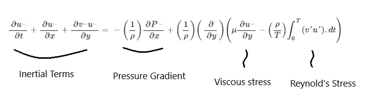
`(delu^_)/(delt)+(delu^_)/(delx)+(delv^_u^_)/(dely)=-(1/rho)(delP^_)/(delx)+(1/rho)(del/(dely))(mu(delu^_)/(dely)-(rho/T)int_0^T(v'u').dt)`

Reynolds stress:

Reynolds stress is the component of the total stress tensor in a fluid obtained from the averaging operation over the Navier–Stokes equations to account for turbulent fluctuations in fluid momentum using Reynolds decomposition. 

One splits the Navier stokes equations into an average and a fluctuating part. One finds that upon averaging the fluid equations, a stress on the right hand side appears of the form `rho \overline {u'_{i}u'_{j}}`. This is the Reynolds stress, conventionally written :

`R_{{ij}}\ \equiv \ \rho \overline {u'_{i}u'_{j}}`

---------------------------------------------------**********------------------------------------------------

##The term shear flow characterizes a flow with a velocity gradient in a direction normal to the mean flow direction: e.g. a boundary layer flow  along a flat plate. In a shear flow, momentum (i.e. momentum per unit volume = ρV) is transferred from the region of high velocity to that of low velocity. The fluid tends to resist the shear associated with the transfer of momentum. The shear stress is proportional to the rate of transfer of momentum.

In laminar flows, the Newton's law  of viscosity relates the shear stress to the rate of angular deformation:

`tau=mu(delu)/(dely)`

Above shear stress `tau` is due to Molecular viscocity(due to interaction of molecules)

where τ is the shear stress, μ is the dynamic viscocity of the flowing fluid, V is the velocity and y is the direction normal to the flow direction. For larger shear stresses, the fluid cannot sustain the viscous shear stress and turbulence spots develop. After apparition of turbulence spots, the turbulence expands rapidly to the entire shear flow. The apparent shear stress in turbulent flow is expressed as:

`tau=rho(nu+nu_T)(delu)/(dely)`

where v is the kinematic viscocity (i.e. v = μ/ρ) and v_T is called the 'Turbulent viscocity' or ‘eddy viscosity’ or momentum exchange coefficient in turbulent flow. The momentum exchange coefficient v_T is a factor depending upon the flow motion. 

Practically, v_T » v in turbulent flows and equation becomes:

`tau=rhonu_T(delu)/(dely)`

#Turbulent viscocity depending upon the flow motion not the fluid.It is greater for flows with more turbulence. 

The turbulent transfer of momentum by eddies giving rise to an internal fluid friction, in a manner analogous to the action of molecular viscocity in laminar flow, but taking place on a much larger scale.

--------------------------------------------**************---------------------------------------------