Literature review - RANS derivation and analysis

AIM

The aim is to conduct a literature review of Reynolds Average Navier Stokes[RANS]

OBJECTIVES

• Derivation of RANS equations
• Performing Reynolds decomposition for engineering flow parameters

REYNOLDS AVERAGED NAVIER STOKES EQUATION

The Reynolds-averaged Navier–Stokes equations (or RANS equations) are time-averaged equations of motion for fluid flow. The idea behind the equations is Reynolds decomposition, whereby an instantaneous quantity is decomposed into its time-averaged and fluctuating quantities, an idea first proposed by Osborne Reynolds.The RANS equations are primarily used to describe turbulent flows. These equations can be used with approximations based on knowledge of the properties of flow turbulence to give approximate time-averaged solutions to the Navier–Stokes equations.

Reynolds Decomposition

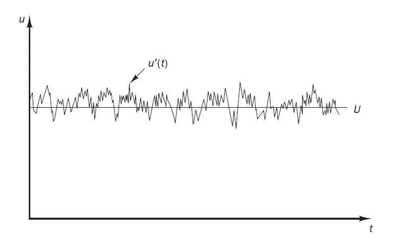
In fluid dynamics and turbulence theory, Reynolds decomposition is a mathematical technique used to separate the expectation value of a quantity from its fluctuations. For example, for a quantity the decomposition would be

where denotes the expectation value of , (often called the steady component/time, spatial or ensemble average), and , are the deviations from the expectation value (or fluctuations). The fluctuations are defined as the expectation value subtracted from quantity such that their time average equals zero. The expected value, , is often found from an ensemble average which is an average taken over multiple experiments under identical conditions. The expected value is also sometime denoted , but it is also seen often with the over-bar notation.

Direct Numerical Simulation, or resolving the Navier-Stokes equations completely , is only possible on small computational grids and small time steps when Reynolds numbers are low. Due to computational constraints, simplifications of the Navier-Stokes equations are useful to parameterize turbulence that are smaller than the computational grid, allowing larger computational domains. Reynolds decomposition allows the simplification the Navier–Stokes equations by substituting in the sum of the steady component and perturbations to the velocity profile and taking the mean value. The resulting equation contains a nonlinear term known as the Reynolds stresses which gives rise to turbulence.

Reynolds Averaging

The three forms most pertinent in turbulence-model research are the

1. Time average,
2. Spatial average
3. Ensemble average

Time averaging is appropriate for stationary turbulence, i.e., a turbulent flow that, on the average, does not vary with time, such as flow in a pipe driven by a constant-speed blower. For such a flow, we express an instantaneous flow variable as f(x, t) . Its time average, FT(x), is defined by

`F_T (x)= lim_(T->oo)1/T int_t^(t + T) f(t,x) dt`

Spatial averaging can be used for homogeneous turbulence, which is a turbulent flow that, on the average, is uniform in all directions. We average over all spatial coordinates by doing a volume integral. Calling the average Fv, we have

`F_V (t)= lim_(V->oo) 1/V intintint_V f(t,x) dV`

Ensemble averaging is the most general type of Reynolds averaging suitable for, e.g., flows that decay in time. As an idealized example, in terms of measurements from N identical experiments (with initial and boundary conditions that differ by random infinitesimal perturbations) where f(x, t) fn(x, t) in the nth experiment, the average is F E• defined by

`F_E(t,x) = lim_(N -> oo)1/N sum_(n=1)^N f_n (t,x)`

RANS DERIVATION

Continuity Equation

`(∂u)/(∂x)+(∂v)/(∂y)=0`

Now, we have to split the instantaneous velocity into mean and fluctuating component

`(∂(baru+u'))/(∂x)+(∂(barv+v'))/(∂y)=0`

`(∂baru)/(∂x)+(∂u')/(∂x)+(∂barv)/(∂y)+(∂v')/(∂y)=0`

Time averaging over time step T

`1/Tint_0^T(∂baru)/(∂x)dt+1/Tint_0^T(∂u')/(∂x)dt+1/Tint_0^T(∂barv)/(∂y)dt+1/Tint_0^T(∂v')/(∂y)dt=0`

Since the fluctuating component is zero

`1/Tint_0^T(∂baru)/(∂x)dt+color(blue)cancel(1/Tint_0^T(∂u')/(∂x)dt)+1/Tint_0^T(∂barv)/(∂y)dt+color(blue)cancel(1/Tint_0^T(∂v')/(∂y)dt)=0`

`1/Tint_0^T(∂baru)/(∂x)dt+1/Tint_0^T(∂barv)/(∂y)dt=0`

Time averaged terms are function of space, we can treat it as constant and remove them from integration

`(∂baru)/(∂x)1/Tint_0^Tdt+(∂barv)/(∂y)1/Tint_0^Tdt=0`

`(∂baru)/(∂x)+(∂barv)/(∂y)=0`

The above equation represents the RANS continuity Equation

Momentum Equation

`ρ[(∂u)/(∂t)+u(∂u)/(∂x)+v(∂u)/(∂y)]=-(∂P)/(∂x)+ μ ((∂^2u)/(∂x^2)+(∂^2u)/(∂y^2))`

Shifting the rho to RHS

`(∂u)/(∂t)+u(∂u)/(∂x)+v(∂u)/(∂y)=-1/rho(∂P)/(∂x)+ ν (∂^2u)/(∂x^2)+ ν (∂^2u)/(∂y^2)`

Lets multiply the x-component of velocity with the continuity equation

`(∂u)/(∂t)+u(∂u)/(∂x)+v(∂u)/(∂y)+u((∂u)/(∂x)+(∂v)/(∂y))=-1/rho(∂P)/(∂x)+ ν (∂^2u)/(∂x^2)+ ν (∂^2u)/(∂y^2)`

`(∂u)/(∂t)+2u(∂u)/(∂x)+v(∂u)/(∂y)+u(∂v)/(∂y)=-1/rho(∂P)/(∂x)+ ν (∂^2u)/(∂x^2)+ ν (∂^2u)/(∂y^2)`

Applying product rule of differentiation

`(∂u)/(∂t)+(∂u^2)/(∂x)+(∂(uv))/(∂y)=-1/rho(∂P)/(∂x)+ ν (∂^2u)/(∂x^2)+ ν (∂^2u)/(∂y^2)`

Now the decomposition step is being done. we get,

`(∂(baru+u'))/(∂t)+(∂(baru+u')^2)/(∂x)+(∂((baru+u')(barv+v')))/(∂y)=-1/rho(∂(barP+P'))/(∂x)+ ν (∂^2(baru+u'))/(∂x^2)+ ν (∂^2(baru+u'))/(∂y^2)`

`(∂baru)/(∂t)+(∂u')/(∂t)+(∂baru^2)/(∂x)+(∂(u')^2)/(∂x)+(∂(2baru u'))/(∂x)+(∂(barubarv))/(∂y)+(∂(baru v'))/(∂y)+(∂(u'barv))/(∂y)+(∂(u'v'))/(∂y)=-1/rho(∂barP)/(∂x)-1/rho(∂P')/(∂x)+ ν (∂^2baru)/(∂x^2)+ ν (∂^2u')/(∂x^2)+ ν (∂^2baru)/(∂y^2)+ ν (∂^2u')/(∂y^2)`

Averaging the time step T and applying integration on both sides

`1/Tint_0^T(∂baru)/(∂t)dt+1/Tint_0^T(∂u')/(∂t)dt+1/Tint_0^T(∂baru^2)/(∂x)dt+1/Tint_0^T(∂(u')^2)/(∂x)dt+1/Tint_0^T(∂(2baru u'))/(∂x)dt+1/Tint_0^T(∂(barubarv))/(∂y)dt+1/Tint_0^T(∂(baru v'))/(∂y)dt+1/Tint_0^T(∂(u'barv))/(∂y)dt+1/Tint_0^T(∂(u'v'))/(∂y)dt=-1/Tint_0^T1/rho(∂barP)/(∂x)dt-1/Tint_0^T1/rho(∂P')/(∂x)dt+ 1/Tint_0^Tν (∂^2baru)/(∂x^2)dt+ 1/Tint_0^Tν (∂^2u')/(∂x^2)dt+ 1/Tint_0^Tν (∂^2baru)/(∂y^2)dt+ 1/Tint_0^Tν (∂^2u')/(∂y^2)dt`

`1/Tint_0^T(∂baru)/(∂t)dt+color(blue)cancel(1/Tint_0^T(∂u')/(∂t)dt)+1/Tint_0^T(∂baru^2)/(∂x)dt+1/Tint_0^T(∂(u')^2)/(∂x)dt+color(blue)cancel(1/Tint_0^T(∂(2baru u'))/(∂x)dt)+1/Tint_0^T(∂(barubarv))/(∂y)dt+color(blue)cancel(1/Tint_0^T(∂(baru v'))/(∂y)dt)+color(blue)cancel(1/Tint_0^T(∂(u'barv))/(∂y)dt)+1/Tint_0^T(∂(u'v'))/(∂y)dt=-1/Tint_0^T1/rho(∂barP)/(∂x)dt-color(blue)cancel(1/Tint_0^T1/rho(∂P')/(∂x)dt)+ 1/Tint_0^Tν (∂^2baru)/(∂x^2)dt+ color(blue)cancel(1/Tint_0^Tν (∂^2u')/(∂x^2)dt)+ 1/Tint_0^Tν (∂^2baru)/(∂y^2)dt+ color(blue)cancel(1/Tint_0^Tν (∂^2u')/(∂y^2)dt)`

The terms which remains are

`1/Tint_0^T(∂baru)/(∂t)dt+1/Tint_0^T(∂baru^2)/(∂x)dt+1/Tint_0^T(∂(u')^2)/(∂x)dt+1/Tint_0^T(∂(barubarv))/(∂y)dt+1/Tint_0^T(∂(u'v'))/(∂y)dt=-1/Tint_0^T1/rho(∂barP)/(∂x)dt+ 1/Tint_0^Tν (∂^2baru)/(∂x^2)dt+ 1/Tint_0^Tν (∂^2baru)/(∂y^2)dt``(∂baru)/(∂t)+(∂baru^2)/(∂x)+1/Tint_0^T(∂(u')^2)/(∂x)dt+(∂(barubarv))/(∂y)+1/Tint_0^T(∂(u'v'))/(∂y)dt=-1/rho(∂barP)/(∂x)+ ν (∂^2baru)/(∂x^2)+ ν (∂^2baru)/(∂y^2)`

Replacing integrals by time average

`(∂baru)/(∂t)+(∂baru^2)/(∂x)+(∂(barubarv))/(∂y)=-1/rho(∂barP)/(∂x)+ ν (∂^2baru)/(∂x^2)+ ν (∂^2baru)/(∂y^2)-(∂(bar(u'v')))/(∂y)-(∂(bar((u')^2)))/(∂x)`

The final momentum equation is

`(∂baru)/(∂t)+(∂baru^2)/(∂x)+(∂(barubarv))/(∂y)=-1/rho(∂barP)/(∂x)+ ν (∂^2baru)/(∂x^2)+ ν (∂^2baru)/(∂y^2)+1/ρ[(∂(-ρbar(u'v')))/(∂y)+(∂(-ρbar((u')^2)))/(∂x)]`

Now the total shear stress can be expressed as

`"Total Shear Stress" = ubrace(μ((∂u_i)/(∂x_j)))_("Laminar Stress")-ubrace(ρ(bar(u_i^')bar(u_j^')))_("Turbulent Stress")`

The Reynolds Stress expression is a tensor quantity as shown below

`τ_(ij)^(Reynolds) = [[τ_(x x), τ_(xy), τ_(xz) ],[τ_(yx), τ_(yy), τ_(yz) ],[τ_(zx), τ_(zy), τ_(zz) ]]=[[-ρbar((u')^2),-ρbar((u'v')),-ρbar((u'w'))], [-ρbar((v'u')),-ρbar((v')^2),-ρbar((v'w'))], [-ρbar((w'u')),-ρbar((w'v')),-ρbar((w')^2)]]`

Reynolds Stress

In fluid dynamics, the Reynolds stress is the component of the total stress tensor in a fluid obtained from the averaging operation over the Navier–Stokes equations to account for turbulent fluctuations in fluid momentum. The velocity field of a flow can be split into a mean part and a fluctuating part using Reynolds decomposition. We write

with being the flow velocity vector having components in the coordinate direction denoting the components of the coordinate vector (). The mean velocities are determined by either time averaging, spatial averaging or ensemble averaging, depending on the flow under study. Further denotes the fluctuating (turbulence) part of the velocity.

We consider a homogeneous fluid, whose density ρ is taken to be a constant. For such a fluid, the components τ'_ij of the Reynolds stress tensor are defined as:

Another – often used – definition, for constant density, of the Reynolds stress components is:

Eddy Viscosity Versus Molecular Viscosity

Joseph Valentin Boussinesq was the first to attack the closure problem, by introducing the concept of eddy viscosity. In 1877 Boussinesq proposed relating the turbulence stresses to the mean flow to close the system of equations. Here the Boussinesq hypothesis is applied to model the Reynolds stress term. Note that a new proportionality constant , the turbulence eddy viscosity, has been introduced. Models of this type are known as eddy viscosity models or EVM's.

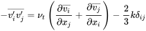
Which can be written in shorthand as

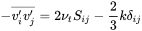
where is the mean rate of strain tensor

is the turbulence eddy viscosity

is the turbulence kinetic energy

and is the Kronecker delta.

In this model, the additional turbulence stresses are given by augmenting the molecular viscosity with an eddy viscosity. This can be a simple constant eddy viscosity (which works well for some free shear flows such as axisymmetric jets, 2-D jets, and mixing layers).

At a molecular level, viscosity is a result the interaction between the different molecules in a fluid. This can be also understood as friction between the molecules in the fluid. Just like in the case of friction between moving solids, viscosity will determine the energy required to make a fluid flow.

CONCLUSION

1. The RANS derivation and analysis was conduced
2. Turbulence model of RANS was interpreted