Centrifugal pump simulation

AIM

The aim of this project is to simulate the flow of liquid inside a centrifugal pump

OBJECTIVES

• Running the simulation with various mass flow rates at outlet
• Increase in outflow distance by twice the impeller diameter
• Performance plot
• Efficiency of pump

CENTRIFUGAL PUMP

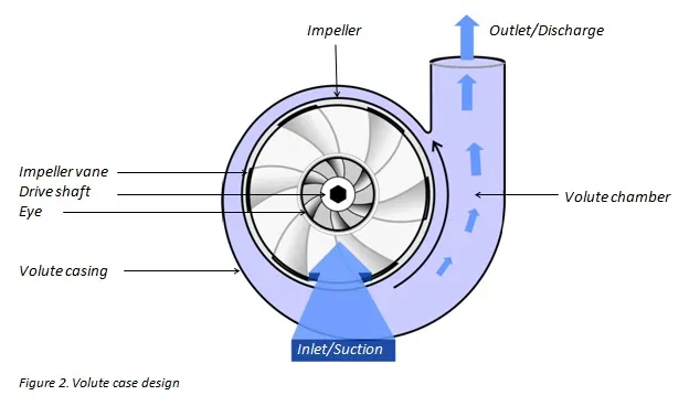
A centrifugal pump is a mechanical device designed to move a fluid by means of the transfer of rotational energy from one or more driven rotors, called impellers. Fluid enters the rapidly rotating impeller along its axis and is cast out by centrifugal force along its circumference through the impeller’s vane tips. The action of the impeller increases the fluid’s velocity and pressure and also directs it towards the pump outlet. The pump casing is specially designed to constrict the fluid from the pump inlet, direct it into the impeller and then slow and control the fluid before discharge.

The impeller is the key component of a centrifugal pump. It consists of a series of curved vanes. These are normally sandwiched between two discs (an enclosed impeller). For fluids with entrained solids, an open or semi-open impeller (backed by a single disc) is preferred.Fluid enters the impeller at its axis (the ‘eye’) and exits along the circumference between the vanes. The impeller, on the opposite side to the eye, is connected through a drive shaft to a motor and rotated at high speed (typically 500-5000rpm). The rotational motion of the impeller accelerates the fluid out through the impeller vanes into the pump casing.

There are two basic designs of pump casing: volute and diffuser. The purpose in both designs is to translate the fluid flow into a controlled discharge at pressure.In a volute casing, the impeller is offset, effectively creating a curved funnel with an increasing cross-sectional area towards the pump outlet. This design causes the fluid pressure to increase towards the outlet.

The same basic principle applies to diffuser designs. In this case, the fluid pressure increases as fluid is expelled between a set of stationary vanes surrounding the impeller (Figure 3). Diffuser designs can be tailored for specific applications and can therefore be more efficient. Volute cases are better suited to applications involving entrained solids or high viscosity fluids when it is advantageous to avoid the added constrictions of diffuser vanes. The asymmetry of the volute design can result in greater wear on the impeller and drive shaft.

SIMULATION OF CENTRIFUGAL PUMP CASE 1 [ MASS FLOW RATE = 130 kg/s]

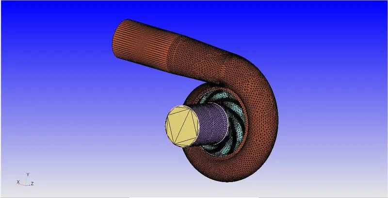
Geometry

Mesh

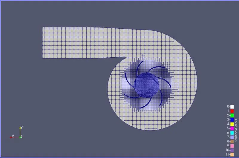
The base mesh size is of 0.012m for the case that has been setup for simulation purpose.The use of AMR can been seen near the impeller blades based on the velocity AMR provided during case setup

Boundary Conditions

Inlet

1. Inflow boundary
2. Pressure = 101325 bar
3. Temperature = 300 K
4. Species - water

Outlet

1. Outflow boundary
2. Mass flow rate = 130 kg/s
3. Temperature = 300 K
4. species - Water

Intake runner

1. Wall boundary
2. Wall motion - Stationary
3. movement - fixed
4. Temperature = 300K

Shroud

1. Wall boundary
2. Wall motion - Stationary
3. movement - fixed
4. Temperature = 300K

Impeller

1. Wall boundary
2. Wall motion - rotating
3. movement - moving
4. Temperature = 300K

Results

Pressure Contour Plot

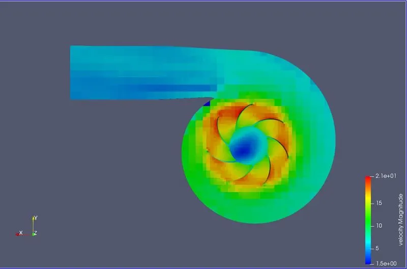
Velocity Contour plot

Pressure plot

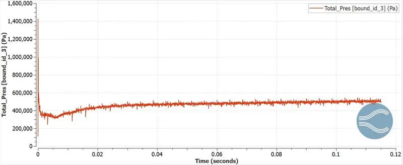
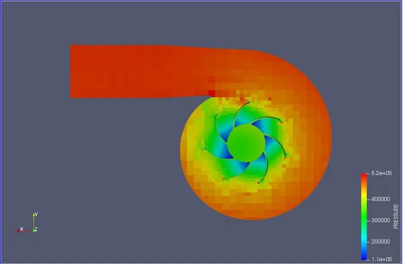
The outlet pressure of the pump with the mass flow rate of 130 kg/s was found out to be 511025 bar. The solution converged to the value that has been showed in the plot.

Velocity Plot

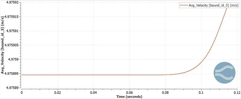
Now in the velocity plot there is a slight increase in the velocity until 4.97592 m/s.

Cell Count

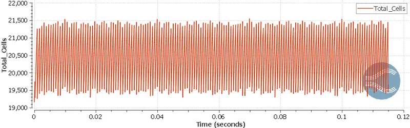
As it is clear from the above plot the cell count max outs at 21500 cells for this simulation case

Pump Efficiency

Pump Efficiency can be calculated by the following formula

Efficiency = Hydraullic power `P_h`/ Shaft power `P_s` x 100

`eta=frac[P_h][P_s]xx100%`

Hydraullic Power

`P_h = frac[QxxH][367] (KW)`

Q - Discharge in `m^3/[hr]`

H - Pressure head in 'm'

`P_h`-Hydraullic power

Discharge is obtained from the mass flow rate of the pump and the pressure head can be obtained by

`H =(Pressure(Pa) xx1e-5)/(0.0981xx S.G.)`

`H = frac[511025xx1e-5][0.0981xx1`

`H = 52.09 m`

Q = 130 x 3.6 `m^3/[hr]`

Q = 468 `m^3/[hr]`

Now the hydraullic power is

`P_h=frac[468xx52.09][367]`

`P_h = 66.42 KW`

Shaft Power

`P_s = Txxomega (KW)`

T - Torque in N-m

`omega`- Angular velocity in rad/sec

`P_s= 354.71xxfrac[2pixx2000][60]`

`P_s = 74.29 KW`

Therefore Pump Efficiency

`eta=66.42/74.29xx100`

`eta=89.42%`

Pressure Animation

Velocity Animation

SIMULATION OF CENTRIFUGAL PUMP CASE 1 [ MASS FLOW RATE = 156 kg/s]

Geometry

Mesh

The base mesh size is of 0.012m for the case that has been setup for simulation purpose.The use of AMR can been seen near the impeller blades based on the velocity AMR provided during case setup

Boundary Conditions

Inlet

1. Inflow boundary
2. Pressure = 101325 bar
3. Temperature = 300 K
4. Species - water

Outlet

1. Outflow boundary
2. Mass flow rate = 156 kg/s
3. Temperature = 300 K
4. species - Water

Intake runner

1. Wall boundary
2. Wall motion - Stationary
3. movement - fixed
4. Temperature = 300K

Shroud

1. Wall boundary
2. Wall motion - Stationary
3. movement - fixed
4. Temperature = 300K

Impeller

1. Wall boundary
2. Wall motion - rotating
3. movement - moving
4. Temperature = 300K

Results

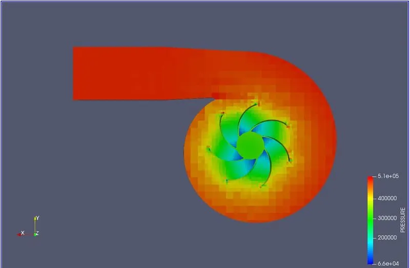
Pressure Contour Plot

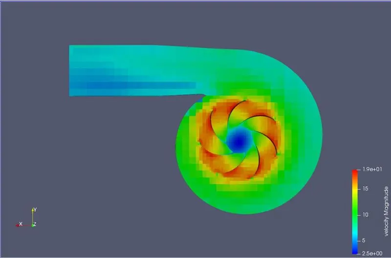
Velocity Contour plot

Pressure plot

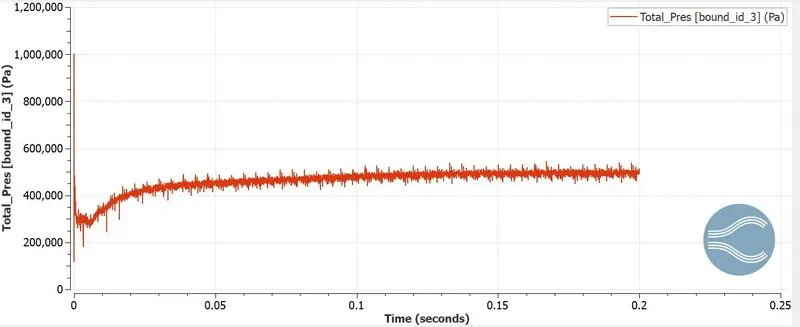
The outlet pressure of the pump with the mass flow rate of 130 kg/s was found out to be 499508 bar. The solution converged to the value that has been showed in the plot.

Velocity Plot

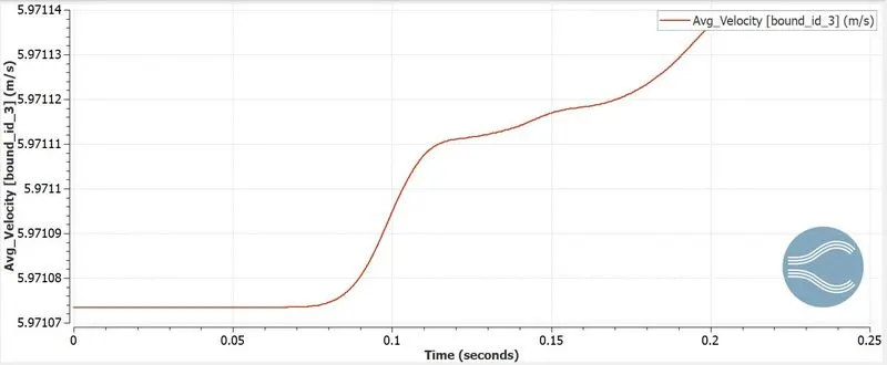
Now in the velocity plot there is a slight increase in the velocity until 5.97114 m/s.

Cell Count

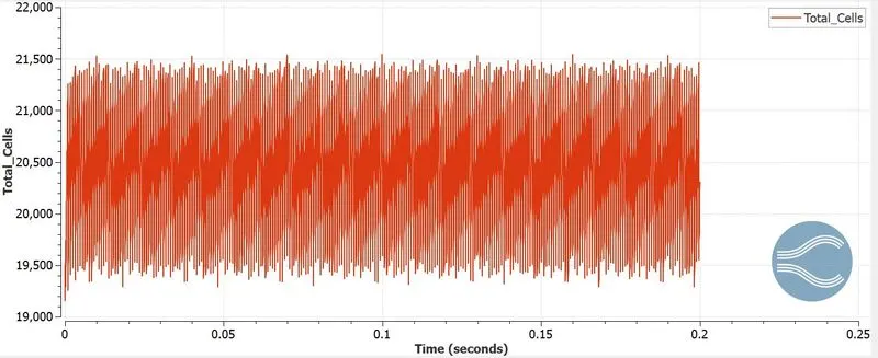
As it is clear from the above plot the cell count max outs at 21500 cells for this simulation case

Pump Efficiency

Pump Efficiency can be calculated by the following formula

Efficiency = Hydraullic power `P_h`/ Shaft power `P_s` x 100

`eta=frac[P_h][P_s]xx100%`

Hydraullic Power

`P_h = frac[QxxH][367] (KW)`

Q - Discharge in `m^3/[hr]`

H - Pressure head in 'm'

`P_h`-Hydraullic power

Discharge is obtained from the mass flow rate of the pump and the pressure head can be obtained by

`H =(Pressure(Pa) xx1e-5)/(0.0981xx S.G.)`

`H = frac[499508xx1e-5][0.0981xx1`

`H = 50.42 m`

Q = 156 x 3.6 `m^3/[hr]`

Q = 561.6 `m^3/[hr]`

Now the hydraullic power is

`P_h=frac[561xx50.42][367]`

`P_h = 77.15 KW`

Shaft Power

`P_s = Txxomega (KW)`

T - Torque in N-m

`omega`- Angular velocity in rad/sec

`P_s= 375.39xxfrac[2pixx2000][60]`

`P_s = 78.62KW`

Therefore Pump Efficiency

`eta=77.15/78.62xx100`

`eta=98.18%`

Pressure Animation

Velocity Animation

SIMULATION OF CENTRIFUGAL PUMP CASE 1 [ MASS FLOW RATE = 180 kg/s]

Geometry

Mesh

The base mesh size is of 0.012m for the case that has been setup for simulation purpose.The use of AMR can been seen near the impeller blades based on the velocity AMR provided during case setup

Boundary Conditions

Inlet

1. Inflow boundary
2. Pressure = 101325 bar
3. Temperature = 300 K
4. Species - water

Outlet

1. Outflow boundary
2. Mass flow rate = 156 kg/s
3. Temperature = 300 K
4. species - Water

Intake runner

1. Wall boundary
2. Wall motion - Stationary
3. movement - fixed
4. Temperature = 300K

Shroud

1. Wall boundary
2. Wall motion - Stationary
3. movement - fixed
4. Temperature = 300K

Impeller

1. Wall boundary
2. Wall motion - rotating
3. movement - moving
4. Temperature = 300K

Results

Pressure Contour Plot

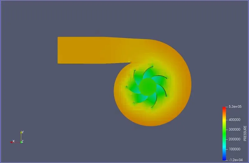
Velocity Contour plot

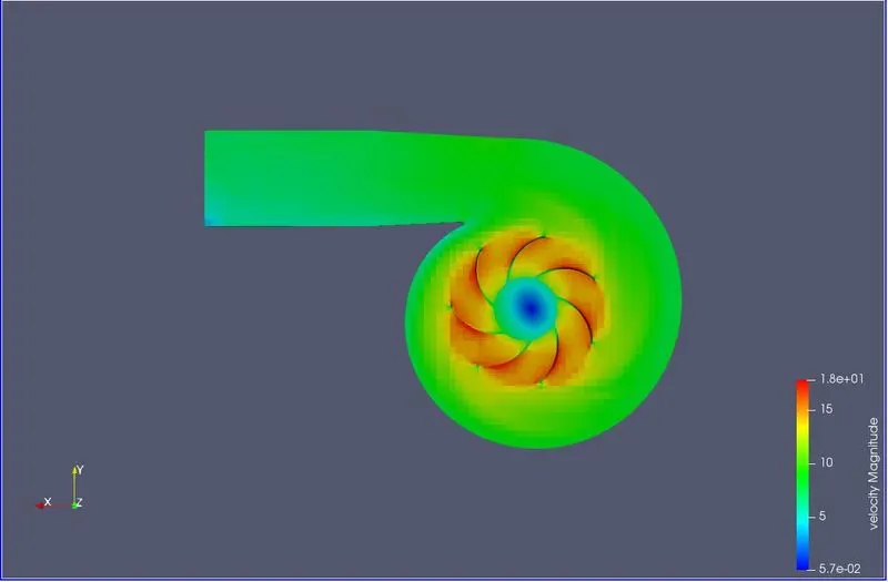
Pressure plot

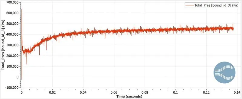
The outlet pressure of the pump with the mass flow rate of 180 kg/s was found out to be 450554 bar. The solution converged to the value that has been showed in the plot.

Velocity Plot

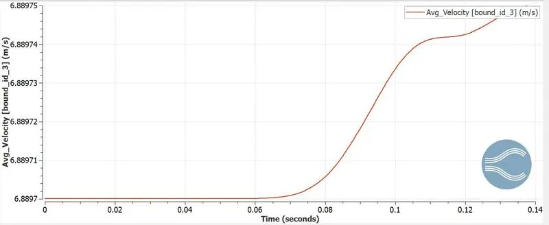
Now in the velocity plot there is a slight increase in the velocity until 6.88975 m/s.

Cell Count

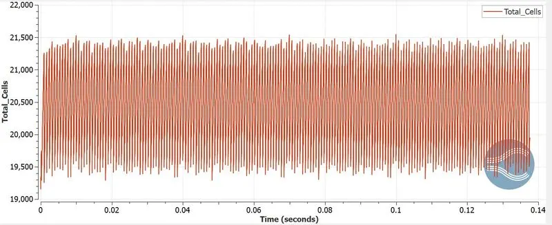
As it is clear from the above plot the cell count max outs at 21500 cells for this simulation case

Pump Efficiency

Pump Efficiency can be calculated by the following formula

Efficiency = Hydraullic power `P_h`/ Shaft power `P_s` x 100

`eta=frac[P_h][P_s]xx100%`

Hydraullic Power

`P_h = frac[QxxH][367] (KW)`

Q - Discharge in `m^3/[hr]`

H - Pressure head in 'm'

`P_h`-Hydraullic power

Discharge is obtained from the mass flow rate of the pump and the pressure head can be obtained by

`H =(Pressure(Pa) xx1e-5)/(0.0981xx S.G.)`

`H = frac[450554xx1e-5][0.0981xx1`

`H = 45.92m`

Q = 180 x 3.6 `m^3/[hr]`

Q = 648 `m^3/[hr]`

Now the hydraullic power is

`P_h=frac[648xx45.92][367]`

`P_h = 81.07 KW`

Shaft Power

`P_s = Txxomega (KW)`

T - Torque in N-m

`omega`- Angular velocity in rad/sec

`P_s= 387.63xxfrac[2pixx2000][60]`

`P_s = 81.18KW`

Therefore Pump Efficiency

`eta=81.07/81.18xx100`

`eta=99.86%`

Pressure Animation

Velocity Animation

PUMP PERFORMANCE CURVE

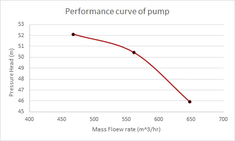
The above plot shows the pump performance curve for all the 3 cases which has been run in this simulation

Pump performance curves are important drawings produced by the pump manufacturer. Pump performance curves are primarily used to predict the variation of the differential head across the pump, as the flow is changed. But in addition variation of efficiency, power, NPSH required etc, as the flow is changed, can also be represented on the pump performance curves by the manufacturer.It is important to be able to read and understand the pump curves for selection, testing, operation and maintenance of pumps.Typically a pump performance curve will carry information about the following points.

Variation of differential head Vs flow

This is the primary information reported in the pump performance curves and very important information regarding most of the pump calculations related to differential pressure across the pump. Differential head Δh is related to differential pressure ΔP by the equation, ΔP = ρgΔh.

It should be note that the pump curves for differential head Vs. volumetric flow rate are plotted for a particular liquid density. If in the future the process liquid or even just liquid density is changed, that effect has to be considered to finally determine the differential pressure. In such as case, revised volumetric flow should be calculated and located on the pump curve and corresponding differential head should be then determined from the curve for the appropriate impeller diameter. This differential head should then be used along with the changed liquid density to determine the differential pressure across the pump.

Pump Efficiency

As indicated in the sample pump performance curve above, the plot of pump efficiency against volumetric flow rate is also commonly reported on the pump performance curves. When the theoretical pumping power requirement is divided by this efficiency for the corresponding flow, the result is pump shaft power requirement. For more information on pump power calculations using efficiency, refer to EnggCyclopedia's solved sample problem. The calculated pump shaft power has to be provided by an electric motor.

1. The pump performance curve was plotted for all 3 cases
2. Efficiency of the pump has been calculated
3. Distance of outflow was increased by twice the size of diameter