Week 8 - BlockMesh Drill down challenge
INTRODUCTION
In this challenge, a geometry is defined and meshed using the blockMesh utility in OpenFoam. The blockMesh utility creates parametric meshes with grading and curved edges. The mesh is generated from a dictionary file named blockMeshDict located in the constant/polyMesh directory of a case. The blockMesh reads this dictionary generates the mesh, and writes out the mesh data to points and faces, cells and boundary files in the same directory.
The principle behind blockMesh is to decompose the domain geometry into a set of 1 or more three dimensional, hexahedral blocks. Edges of the blocks can be straight lines, arcs or splines. The mesh is ostensibly specified as a number of cells in each direction of the block, sufficient information for blockMesh to generate the mesh data.
Each block of the geometry is defined by 8 vertices, one at each corner of a hexahedron. The vertices are written in a list so that each vertex can be accessed using its label, remembering that OpenFOAM always uses the C++ convention that the first element of the list has the label ‘0’.
The geometry that needs to have meshed is of a backward-facing step. The effect of grading on the velocity is also analyzed. The flow through the backward-facing step produces a flow separation region and a recirculation zone. The effects can be taken care of by using a solver that can handle turbulence. So the simpleFoam solver is selected for this problem. SimpleFoam is a steady-state solver for incompressible, turbulent flow, using the SIMPLE (Semi-Implicit Method for Pressure Linked Equations) algorithm.
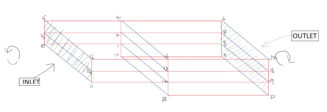
The geometry to be defined is shown below:
THE blockMeshDict
The blockMeshDict file defining the given geometry is shown below:
/*--------------------------------*- C++ -*----------------------------------*\
  =========                 |
  \\      /  F ield         | OpenFOAM: The Open Source CFD Toolbox
   \\    /   O peration     | Website:  https://openfoam.org
    \\  /    A nd           | Version:  8
     \\/     M anipulation  |
\*---------------------------------------------------------------------------*/
FoamFile
{
    version     2.0;
    format      ascii;
    class       dictionary;
    object      blockMeshDict;
}
// * * * * * * * * * * * * * * * * * * * * * * * * * * * * * * * * * * * * * //

// Note: this file is a Copy of $FOAM_TUTORIALS/resources/blockMesh/pitzDaily

convertToMeters 0.01;

vertices
(
    (0 0 0) //vertex 0
    (8 0 0) //vertex 1
    (8 0.5 0) // vertex 2
    (0 0.5 0) // vertex 3
    (8 1 0) // vertex 4
    (0 1 0)  // vertex 5
    (20 1 0) // vertex 6
    (20 0.5 0) // vertex 7
    (20 0 0) // vertex 8
    (20 -1 0) // vertex 9
    (8 -1 0) // vertex 10

    (0 0 0.1) //vertex 11
    (8 0 0.1) //vertex 12
    (8 0.5 0.1) // vertex 13
    (0 0.5 0.1) // vertex 14
    (8 1 0.1) // vertex 15
    (0 1 0.1)  // vertex 16
    (20 1 0.1) // vertex 17
    (20 0.5 0.1) // vertex 18
    (20 0 0.1) // vertex 19
    (20 -1 0.1) // vertex 20
    (8 -1 0.1) // vertex 21

);


blocks
(
    hex (0 1 2 3 11 12 13 14) (200 10 1) simpleGrading (0.2 1.2 1)
    hex (3 2 4 5 14 13 15 16) (200 10 1) simpleGrading (0.2 0.2 1)
    hex (2 7 6 4 13 18 17 15) (200 10 1) simpleGrading (1.2 0.2 1)
    hex (1 8 7 2 12 19 18 13) (200 10 1) simpleGrading (1.2 1.2 1)
    hex (10 9 8 1 21 20 19 12) (200 10 1) simpleGrading (1.2 1.2 1)
);

edges
(
);

boundary
(
    inlet
    {
        type patch;
        faces
        (
            (0 11 14 3)
            (3 14 16 5)
        );
    }
    outlet
    {
        type patch;
        faces
        (
            (9 8 19 20)
            (8 7 18 19)
            (7 6 17 18)
        );
    }
    upperWall
    {
        type wall;
        faces
        (
            (16 15 4 5)
            (15 17 6 4)
        );
    }
    lowerWall
    {
        type wall;
        faces
        (
            (1 10 21 12)
            (0 1 12 11)
            (9 20 21 10)
        );
    }
    frontAndBack
    {
        type empty;
        faces
        (
            (15 13 14 16)
            (13 12 11 14)
            (17 18 13 15)
            (18 19 12 13)
            (19 20 21 12)
            (4 2 3 5)
            (2 1 0 3)
            (6 7 2 4)
            (7 8 1 2)
            (8 9 10 1)
        );
    }
);

// ************************************************************************* //
The mesh generated using the blockMesh utility can be visualised using paraview, which is given below:
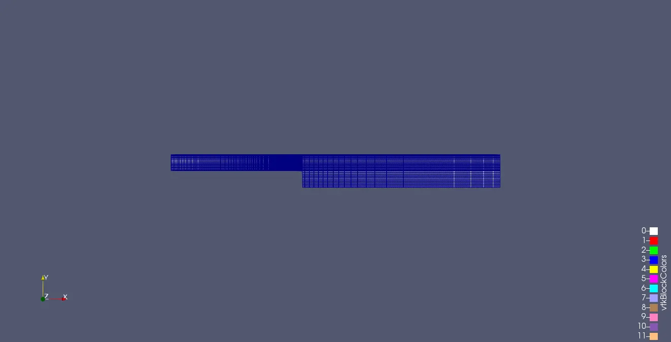
The above blockMeshDict file was created by editing an existing tutorial case, whwere a similar problem is solved using the simpleFoam solver. The case Iused for the study was pitzDaily. The other files were used as such without any edits. The postprocessing is carried out using paraview as well as python. The velocity contours and streamlines were also visualised using paraview.
The grading can be changed by changing some lines of code in the blockMeshDict as shown below. For the grading factor near the walls to be 0.5
blocks
(
    hex (0 1 2 3 11 12 13 14) (200 10 1) simpleGrading (0.5 1.5 1)
    hex (3 2 4 5 14 13 15 16) (200 10 1) simpleGrading (0.5 0.5 1)
    hex (2 7 6 4 13 18 17 15) (200 10 1) simpleGrading (1.5 0.5 1)
    hex (1 8 7 2 12 19 18 13) (200 10 1) simpleGrading (1.5 1.5 1)
    hex (10 9 8 1 21 20 19 12) (200 10 1) simpleGrading (1.5 1.5 1)
);
For the grading factor near the walls to be 0.8
blocks
(
    hex (0 1 2 3 11 12 13 14) (200 10 1) simpleGrading (0.8 1.8 1)
    hex (3 2 4 5 14 13 15 16) (200 10 1) simpleGrading (0.8 0.8 1)
    hex (2 7 6 4 13 18 17 15) (200 10 1) simpleGrading (1.8 0.8 1)
    hex (1 8 7 2 12 19 18 13) (200 10 1) simpleGrading (1.8 1.8 1)
    hex (10 9 8 1 21 20 19 12) (200 10 1) simpleGrading (1.8 1.8 1)
);
RESULTS AND DISCUSSION
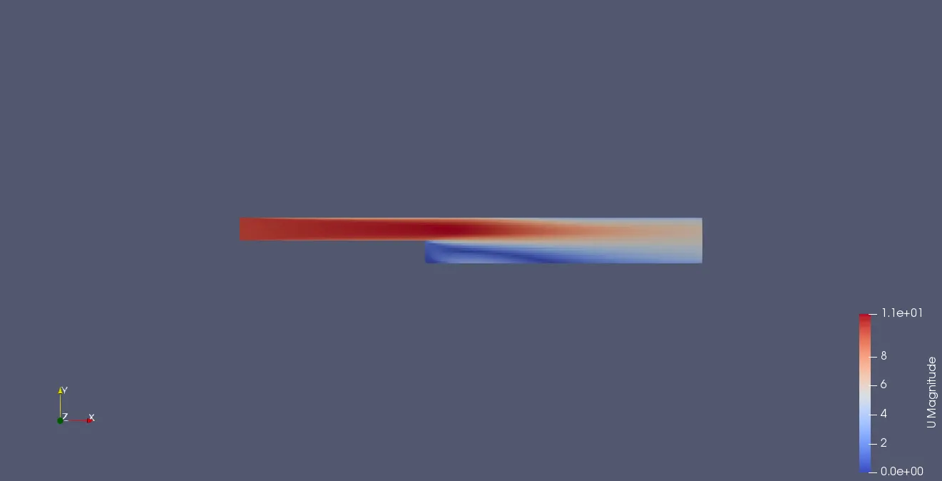
The velocity contour for the wall grading factor of 0.2 is shown below:
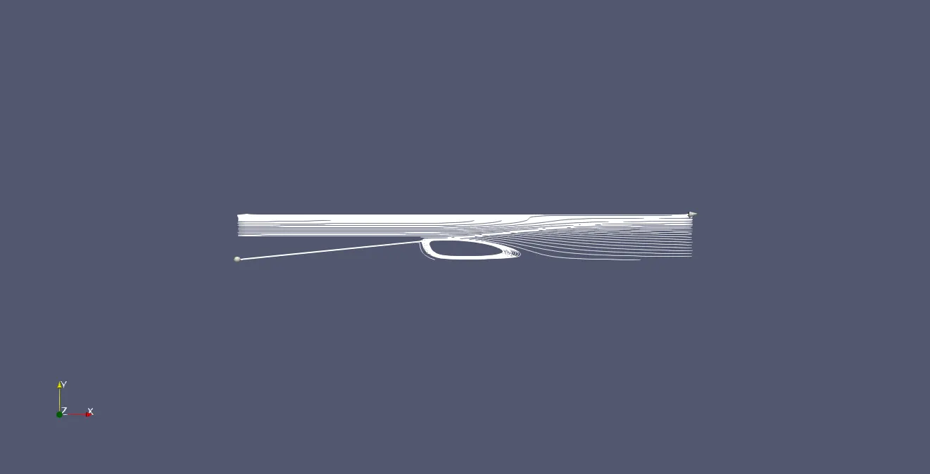
The streamline plot is shown below for grading factor = 0.2
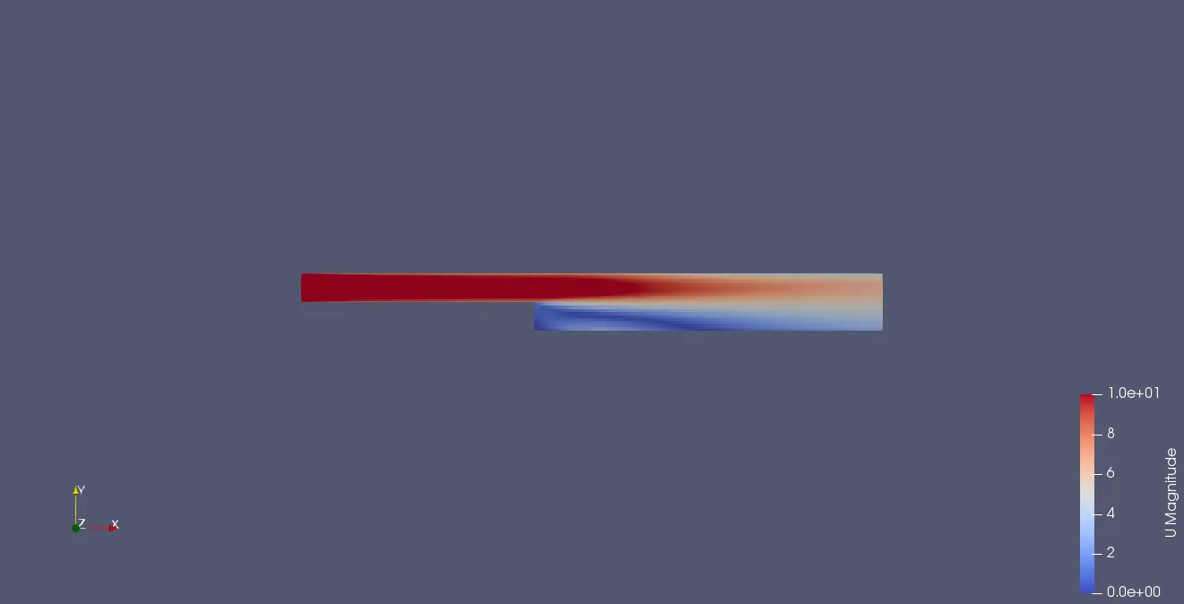
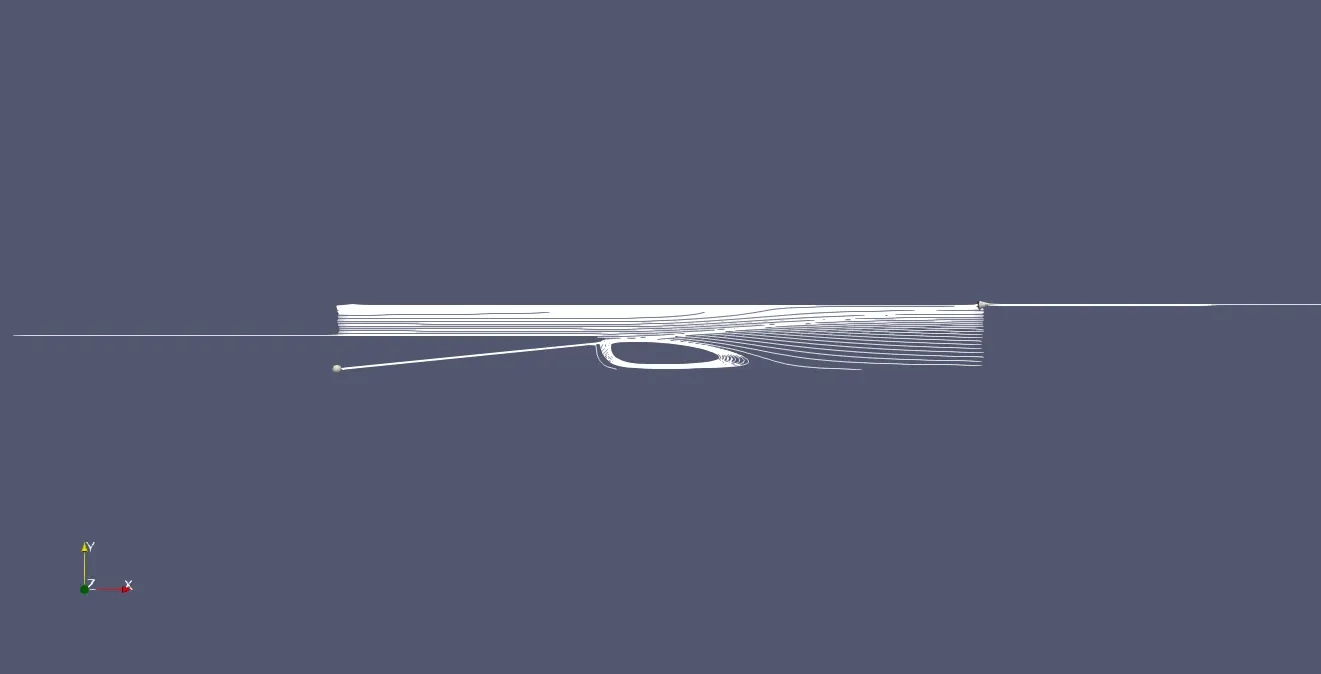
The velocity contour and the streamlines when the grading factor is 0.5 is shown below:
The velocity contour is shown below:
The streamlines are shown below:
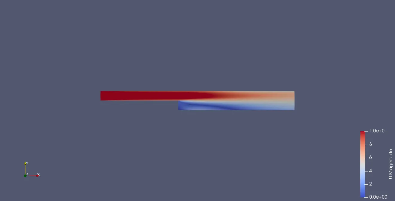
The velocity and streamline plots for grading factor = 0.8 is shown below:
The velocity contour is shown below:
The streamline plot is shown below:
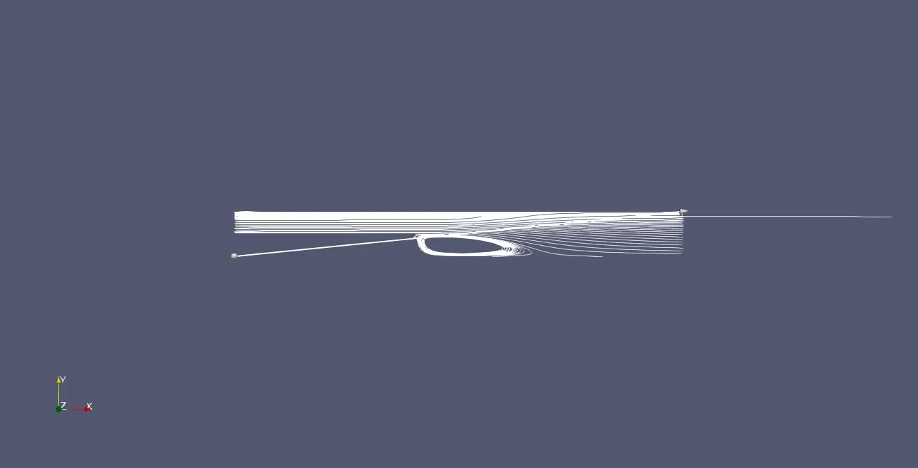
The velocity contours and stereamlines for the different grading factor seems to be similar. The effectof grading can be analysed comparing he velocity magnitude at a distance of x = 0.08 m from the inlet. The csv files for different cases were extracted from paraview using the plot over line filter and the plot is generated using the matplotlib library in python.
The comparison of velocity magnitude at x = 0.085m from the inlet for the different wall grading factor is shown below:
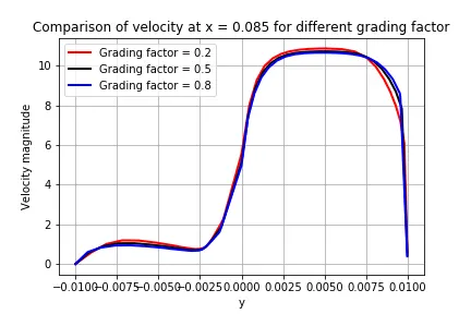
From the above figure it can be seen that grading has very small effect on the solution.
CONCLUSION
The solution of the bacward facing step has little effect on thegrading provided.
The recirculation zone generated was captured which was visualised using streamlines.
The comparison of velocity at x = 0.08 m was plotted using matplotlib library in python and there was very small variations found