Week 7 State of charge estimation

1. Battery Management System:

Battery Management System (BMS) is any electronic system that manages a rechargeable battery, such as by protecting the battery from operating outside its safe operating area, monitoring its state, calculating secondary data, reporting that data, controlling it's environment, authenticating it and balancing it. A battery pack built together with a battery management system with an external communication data bus is a smart battery pack. A smart battery pack must be charged by a smart battery charger.

Function of BMS:

A BMS may monitor the state of the battery as represented by various items, such as:

1) Voltage: Total voltage, Voltages of individual cells or voltage of periodic taps.

2) Temperature: Average temperature, coolant intake temperature, coolant output temperature and temperatures of individual cells.

3) Coolant flow: For liquid cooled batteries.

4) Current: Current in or out of the battery.

5) Health of individual cells.

6) State of balance of cells.

The BOM will also control the recharging of the battery by redirecting the recovered energy, that is from regenerative braking back into the battery pack (typically composed of a number of battery modules, each composed of a number of cells. Battery thermal management systems can be either passive or active and the cooling medium can either be air, liquid or some form of phase change. AAir cooling is advantageous in its simplicity. Such systems can be passiverelying on the convection of the surrounding air, or active using fans for airflow. The major disadvantage of air cooling is its inefficiency. Large amounts of power must be used to operate the cooling mechanism, far more than active liquid cooling. The additional components of the cooling mechanism also add weight to the BMS, reducing the efficiency of batteries used for transportation. Liquid cooling has a higher natural cooling potential than air cooling as liquid coolants tend to have higher thermal conductivities than air. The batteries can either be directly submerged in the coolant or coolant can flow through the BMS without directly contacting the battery. Indirect cooling has the potential to create large thermal gradients across the BMS due to the increased length of the cooling channels. This can be reduced by pumping the coolant faster through the system, creating a tradeoff between pumping speed and thermal consistency.

Computation:

A BMS my calculatee values based on below parameters, such as:

• Voltage: Minimum and maximum cell voltage.
• State of Charge (SoC) or Depth of Discharge (DoD): to indicate the charge level of the battery.
• State of Health (SoH): A variously defined measurement of the remaining capacity of the battery as percentage (%) of the original capacity.
• State of Power (SoP): The amount of power available for a defined time interval given the current power usage, temperature and other conditions.
• State of Safety (SoS).
• Maximum charge current as a charge current limit (CCL).
• Maximum discharge current as a discharge current limit (DCL).
• Energy [kWh] delivered since last charge or charge cycle.
• Internal impedance of a cell (to determine open circuit voltage).
• Charge (Ah) delivered or stored sometimes this feature is called Coulomb counter.
• Total energy delivered since first use.
• Total operating time since first use.
• Total number of cycles.
• Temperature Monitoring.
• Coolant flow for air or liquid cooled batteries.

Communication:

The central controller of a BMS communicates internally with its hardware operating at a cell level, or externally with high level hardware such as laptops or an HMI. High level external communication are simple and use several methods:

• Different types of serial communications.
• CAN bus communications, commonly used in automotive environments.
• Different types of wireless communications.

Low voltage centralized BMSes mostly do not have any internal communications. Distributed or modular BMSes must use some low level internal cell-controller (Modular architecture) or controller-controller (Distributed architecture) communication. These types of communications are difficult, especially for high voltage systems. The problem is voltage shift between cells. The first cell ground signal may be hundreds of volts higher than the other cell ground signal. Apart from software protocols, there are two known ways of hardware communication for voltage shifting systems, optical-isolator and wireless communication. Another restriction for internal communications is the maximum number of cells. For modular architecture most hardware is limited to maximum 255 nodes. For high voltage systems the seeking time of all cells is another restriction, limiting minimum bus speeds and losing some hardware options. Cost of modular systems is important, because it may be comparable to the cell price. Combination of hardware and software restrictions results in a few options for internal communication:

• Isolated serial communications.
• wireless serial communications.

Protection:

A BMS may protect its battery by preventing it from operating outside its safe operating area, such as:

• Over-charging
• Over-discharging
• Over-current during charging
• Over-current during discharge
• Over-voltage during charging especially important for lead-acid, Li-ion and LiFePO4 cells.
• Under-voltage during discharging, especially important for Li-ion and LiFePO4 cells.
• Over-temperature
• Charging while under low temperature
• Over-pressure
• Ground fault or leakage current detection

The BMS may prevent operation outside the battery's safe operating area by:

• Including an internal switch which is opened if the battery is operated outside its safe operating area.
• Requesting the devices to which the battery is connected to reduce or even stop using or charging the battery.
• Actively controlling the environment, such as through heaters, fans, air conditioning or liquid cooling. 

Battery Connection:

A BMS may also feature a precharge system allowing a safe way to connect the battery to different loads and eliminating the excessive inrush currents to load capacitors. The connection to loads is normally controlled through electromagnetic relays called contactors. The precharge circuit can be either power resistors connected in series with the loads until the capacitors are charged. Alternatively, a switched mode power supply connected in parallel to loads can be used to charge the voltage of the load circuit up to a level close enough to battery voltage in order to allow closing the contactors between battery and load circuit. A BMS may have a circuit that can check whether a relay is already closed before precharging (due to welding for example) to prevent inrush currents to occur.

Figure (1) below shows the block diagram of BMS Main Controller.

                                                                      

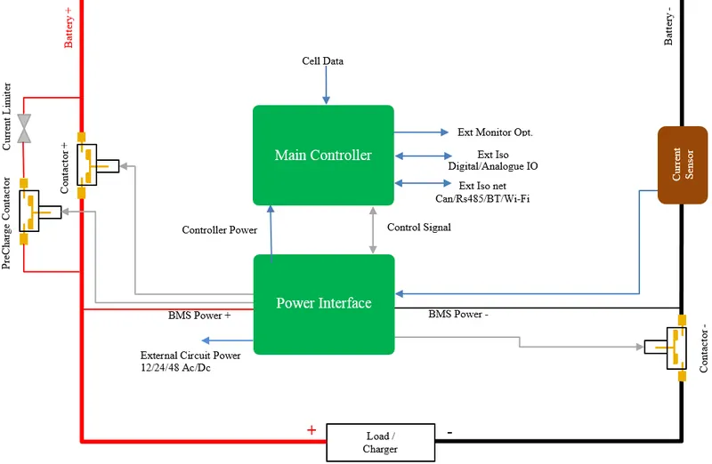
                                                                             Figure (1): BMS Main Controller.

Balancing:

In order to maximize the battery's capacity, and to prevent localized under-charging or over-charging, the BMS may actively ensure that all the cells that compose the battery are kept at the same voltage or State of Charge, through balancing. The BMS can balance the cells by:

• Wasting energy from the most charged cells by connecting them to a load, such as through passiveregulators.
• Shuffling energy from the most charged cells to the least charged cells.
• Reducing the charging current to a sufficiently low level that will not damage fully charged cells, while less charged cells may continue to charge. This does not apply to Lithium chemistry cells.

Topologies of BMS:

BMS technology varies in complexity and performance:

• Simple passive regulators achieve balancing across batteries or cells by bypassing charging current when the cell's voltage reaches a certain level. The cell voltage is a poor indicator of the cell's SoC (and for certain lithium chemistries, such as LiFePO4, it is no indicator at all), thus, making cell voltages equal using passive regulators does not balance SoC, which is the goal of a BMS. Therefore, such devices, while certainly beneficial, have severe limitations in their effectiveness.
• Active regulators intelligently turning on and off a load when appropriate, again to achieve balancing. If only the cell voltage is used as a parameter to enable the active regulators, the same constraints noted above for passive regulators apply.
• A complete BMS also reports the state of the battery to a display, and protects the battery.

BMS topologies fall in three categories:

• Centralized: a single controller is connected to the battery cells through a multitude of wires
• Distributed: a BMS board is installed at each cell, with just a single communication cable between the battery and a controller
• Modular: a few controllers, each handling a certain number of cells, with communication between the controllers

Centralized BMSs are most economical, least expandable, and are plagued by a multitude of wires. Distributed BMSs are the most expensive, simplest to install, and offer the cleanest assembly. Modular BMSes offer a compromise of the features and problems of the other two topologies. The requirements for a BMS in mobile applications, such as electric vehicles and stationary applications like stand-by UPSes in a server room are quite different, especially from the space and weight constraint requirements, so the hardware and software implementations must be tailored to the specific use. In the case of electric or hybrid vehicles, the BMS is only a subsystem and cannot work as a stand-alone device. It must communicate with at least a charger or charging infrastructure, a load, thermal management and emergency shutdown subsystems. Therefore, in a good vehicle design the BMS is tightly integrated with those subsystems. Some small mobile applications, such as medical equipment carts, motorized wheelchairs, scooters, and fork lifts often have external charging hardware, however the on-board BMS must still have tight design integration with the external charger.

In this excercise, we are going to simulate BMS plant with various test cases. To know about the test cases, we have to know about the BMS (Battery Management System) working plant and also BMS ECU (Electronic Control Unit) which is the software simulation environment. By this simulation of BMS model, we can also balance the model by using balance logic which is present in BMS ECU.

The BMS model for simulation is beiing downloaded from the link provided below:

"https://in.mathworks.com/matlabcentral/fileexchange/72865-design-and-test-lithium-ion-battery-management-algorithms".

After downloading the model, we need to follow certain steps for simulation of the BMS model. Figure (2) shows files of BMS system for simulation. We need to extract the zip file which was downloaded from Mathworks website.

                                

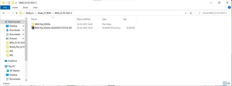
                                                            Figure (2): BMS Simulation files

BMS Project file:

After extracting the file, when we click on the file, we would find the entire project for BMS simulation. We need to click on the "Plant" file as shown in figure (3) below.

                       

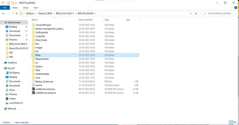
                                                                                Figure(3): BMS Extracted Files

Now, we need to open the "Battery Model" simulink file in which when opened, we can seebelow in figure (4). From the plant sub system, we can observe the main parts are, battery pack, pre charge circui, charger load and their internal connections as closed loop for the feedback purpose.

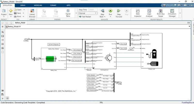
                                          Figure(4): Battery Model.

The BMS model is a ombination of various subsystem models. The models consisted the following parts:

i) The BMS ECU.

ii) BMS Plant.

iii) The test harness Dashboard (Closed Loop).

BMS Plant:

By clicking on the BMS plant subsystem in the BMS model, we get the BMS plant simulink model which is shown below in figure (4). From figure (4), we can observe the main parts of BMS plant are, battery pack, pre charge circuit, charger load and their internal connections as closed loop for the feedback purpose. The battery pack in the plant model have the input as balance command from the BMS and have the outputs as cell level voltage, total pack voltage, total pack current, cell temperatures and battery positive and negative terminals. The inner subsystems or ports or the blocks in the battery pack are shown in figure (5).

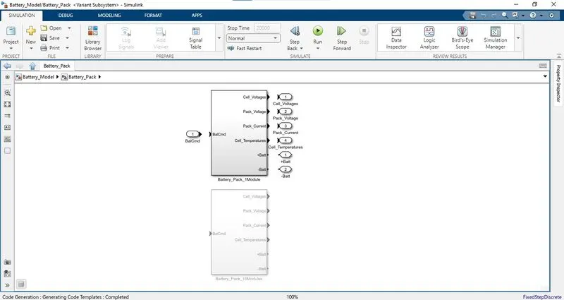
                                          Figure (5): Battery Pack

The battery  pack mainly consists of two types of battery pack module which have six cells in one module that ar connected in series to each other which have six positive terminals of each cell and one negative terminal which goes to ground. The voltage in each cell is calculated as total pack voltage and the current remains same. The other type is having the battery pack of 16 modules which having 16 modules connected to the battery pack of each having 6 cells which all are connected in series so the total cells are 96 connected in series to each other in this also having the cell level voltage, pack voltage and the pack current cell temperature is calculated for each cell in 1 and 16 module. This positive and negative terminals are connected between the charge or load and battery to not affect by over charge and over current which act as a transistor. The inner part of pre charger circuit is shown in figure (6) below.

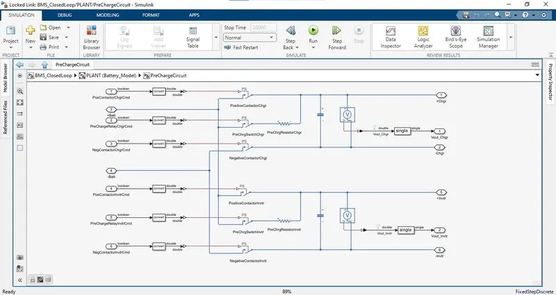
                                         Figure (6): Precharger Circuit

The pre charger switch is connected in between the positive and negative conductor charger with the pre charge resistor in the charge side. As the same in the inverter side also the pre charger is connected between positive and negative contactor through resistor. Based on the given condition the charger or the inverter are connected through the resistor. When the negative contactor is connected, current flows to the pre charged switch after that it flows to positive contactor charge through the high levelled resistor for time delay operations if there is any fault observed in this circuit the pre charged is disconnects and it cut off with the positive contactor for protection purpose. The next is the charger load which is used to connect to the battery for charging through the charger and to discharge through the load. The inner part of the charger load having the charger and the driver load with their internal connections connected in parallel. Based on given state request the connections are made and there connectrespectively. The blocks of the inner circuit of the charger load is given below figure (7).

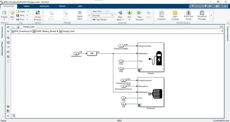
                                                     Figure (7): Charger Load Circuit

BMS ECU:

The full form of BMS ECU is Battery Management System Electronic Control Unit. It is a simple BMS software which is used to run the battery functionalities without errors. These functionalities or the programmes are implemented at state machine diagram which is placed in the BMS ECU which is shown in figure (8).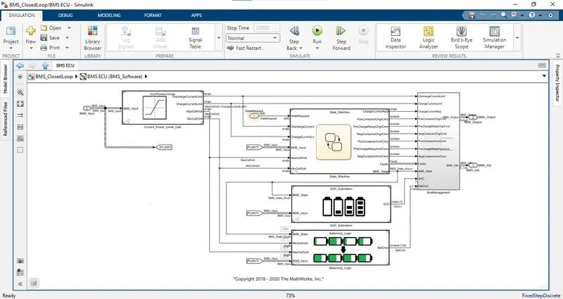 

                                                      Figure (8): BMS ECU

In this block, we can see that the main parameters were the current power limits calculator, state machine, SOC estimation, balancing logic, bus management. From all the parameters the state machine is the main part which is the brain of the BMS ECU. Figure (9) shows the state machine of BMS ECU.

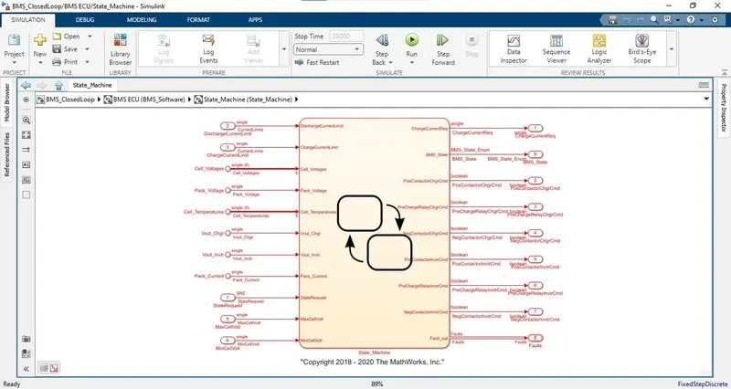
                                  Figure (9): BMS ECU State Machine

As the name indicates, it works as the brain that is, it takes the decision of controls of BMS, faults detections, it's internal conditions, etc. It takes the inputs as current limits, cell and pack voltages, cell temperatures, charger and inverter voltage outputs, pack current, state request, maximum and minimum cell voltages. After the logical operations or algorithm functions are completed based on the given inputs the output is taken from other side of the state machine those are, required charge current, BMS state, pre-charge relay charger and inverter command, positive contactor charger and inverter command, negative contactor charger and inverter command, faults output. It is used to calculate the charge and discharge currents based on the given inputs. The flow chart of the state machine is shown in figure (10).

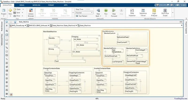
                Figure (10): BMS ECU State Machine Flow Chart

From the flow chart shown in figure (10), it is observed that how a state machine works. For every work there been a separate blocks like main state machine, for fault monitoring for charge contactor state and for inverter contactor state. The State of Charge estimation block is shown in figure (11).

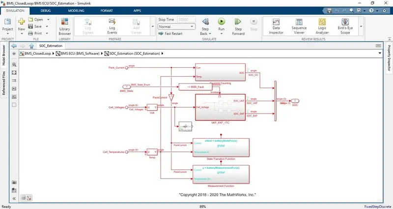
                                   Figure (11): SOC Estimation Block

Here, as per figure (11), by using the pack current, cell voltage and cell temperature we are finding the SOC.

Test Harness Dashboard:

The test harness dashboard is the model which is used to test the BMS model outputs by changing the values of the given input to the BMS. By changing the values of the test conditions, we can observe the results in the form of the graph in the scope. The model of the test hardness model is shown in figure (12).

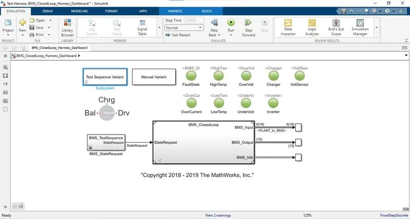
                               Figure (12): BMS Test Harness Dashboard.

In this model the lights which are in green colour used to indicate the fault conditions, when faults are occurred in the model by the given input these led lights blink in the red colour which indicates fault state. The faults that are detecting in this model are fault state, over current, high temperature, low temperature, over voltage, under voltage, charger, inverter, voltage sensor. There are three operating conditions in this model which the battery, they are Driving, charging and balancing. There are three test case conditions in this model, which is used to find out the results those are chosen by the test sequency variant sub system which is shown in figure (13).

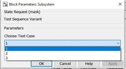
                           Figure (13): Test Cases

As per figure (13), we need to select the test case, the inputs are given. We can see this in the BMS state request by clicking in the BMS test sequence. Figure (14) shows the test sequence editor window for test case1.

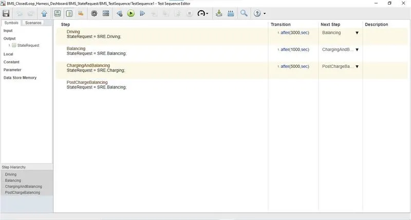
            Figure (14): BMS Test Case 1 Test Sequence Editor

From figure (14), the simulation is running for 2000 seconds. Here, for 3000 seconds the vehicle is in driving condition, after that, from 3001 to 4000 seconds, the BMS is running the balancing condition and finally from 4001 to 9000 seconds, the BMS is charging the battery and starts balancing again from 9001 to 20000 seconds. By cliicking on the run by keeping the stop time as 20000 seconds, we get the results in the scope as a graph and the test harness model looks like in the figure (15) shown below.

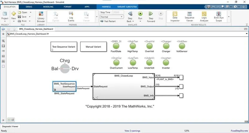
                 Figure (15): BMS Harness Dashboard after simulation with test sequence 1

From figure (15), we observe that the LEDs are indicating green colour. This means that there are no issues in the model so the simulation ran without fault. The graphical representation of the given condition is given in figure (16).

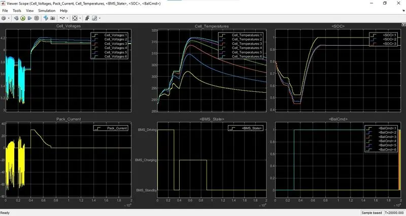
                                                 Figure (16): Test Condition 1 Scope Results.

The graphs that are plotted in figure (16) are cell voltage, pack current, cell temperature, BMS state, state of charge and balance command. If we observe the cell voltages graph, each cell is indicated by the different colour for identification. The cell voltage of all cells in the entire battery pack, while simulating the model the cell voltages are changing as per the current flow. In the initial stage of the simulation the voltages are slightly different because the model simulation was initialized with a slight associate of imbalance in the voltages are directing from 3.1V to 3.9V. Now we can visualize the balance state of voltages their respective cells until the voltage of cells reach 4.2V and it will remain till the end of the simulation. We can observe a small voltage difference in their voltages and the voltage lies between 4V to 4.2V due to the system is on standby mode. Here if we observe from 0 to 3000 sec the voltage in fluctuates that is up and down from the 3.9 to 3.1 V which is their discharge limits. These are plotted due the driving condition. From 3001 to 4000 sec, it is in balance condition hence it is in constant state at 3.6 to 3.9V. after that from 4001 to 9000 sec the state was the charging state. at this condition the constant current (CC) and constant voltage (CV) are occur, at start CC are with very less time after that CV occur for the time longer than the CC. after charging was completed it changes to balance condition due to the balancing system. From 9001 to 20000 sec again the condition was the balancing condition due to this it remains constant up to 20000 sec.

If we observe in the cell temperature, we can observe different temperatures for differeent cells due to the location in the battery pack. and their construction. If we observe here that in driving condition, the temperature increased based on the driving conditions but in the balance condition it gets  to slow down which means the battery temperature is cooling (Individual cells). Again, in the charging condition, it reaches to the highest ranges which we can conclude that during charging, battery gets more heat. Again, during or after balancing condition, it reduces its temperature and tries to gets normal. In detail, if we want observation on cell temperature, the temperature starts at 289 degrees and it will increases gradually, all the cells have different temperatures. The temperature traces shows the significant difference between the highest and lowest temperature cells, due to symmetry in the merged layers in terms of their thermal characteristics and behaviour. The 6^th cell is high temperature cell and the 1^st cell is lowest temperature cell due to it is thermally insulated at one side. In the graph we can visualize that the temperature of the cells will gradually increase till the time of 0.6*10^4 seconds and then the temperatures of all the cells will stars depleting gradually, at the end of the simulation the temperatures of all the cells are 293 degrees, 297 degrees, 302 degrees,.304.95 degrees, 307 degrees and 308 degrees.

If we observe the current graph, the fluctuations are occurred due to driving condition from 0 to 3000 seconds. It is from 20A to -65A. From 3000 to 4000sec, the balancing is placed due to this the current is 0A. From 4001 to 9000sec it gets charging due to this at start it was CC with 30A current value. It gets decreased once the CV mode kicks in, and decreases to 0A. After 9000 sec due to balancing condition it again placed in 0A value upto 20000sec.

The SOC (state of charge) graph visualizes the differnt battery cell performances corresponding to coulomb count method, corresponding to ukf and ekf. The initial SOC is 75%, the starts at 80% to set their capability to recover. It is apparent that coulomb counting never does, because it has no way to get feedback to understand it is wrong due to its absence of voltage information. Both the algorithms recover on the other hand, from the initial error within the first hour of simulated time. With the ekf slightly outperforming than ukf. In the SOC graph the coulomb counting is different and SOC UKF and EKF SOC conditions are plotted as near to each other in this the coulomb counting is little high but the SOC UKF and EKF are perfect or accurate than coulomb. If we observe the graph that the battery SOC is at the range of 80% at the starting. Due to driving the discharge of the battery occur and it reduced to 45 to 50%, in balancing condition it remains constant. Now due to charging occurred it started charging if we observe here at staring stage of charging it gets charged faster after that it takes due to CC and CV respectively. When it gets charged it takes the constant position from 7000 to 9000 sec. after that due to balancing condition it again in the constant mode.

In the BMS state it is simple to understand that when the state is getting activated it gets in the constant after that it getting to 0. If we see here in the starting the driving is on up to 3000 sec after that the balancing takes place stand by is on. When charging is going BMS charging is on and again for balancing the stand by in getting on.

Test Condition 2:

In the second test condition, there is only driving and cherging phase that is for 20000 seconds. Figure (17) shows the selection of test case 2 in Simulink Harness Dashboard model.

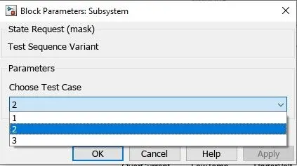
                        Figure (17): Test Case 2 Selection

As per above figure (17), we have selected test case 2 and run the model for 20000 seconds. After running the model successfully, in the dashboard we can visualize that two lamp blocks will show red colour. This indicates that while running the test case two the simulation have gone through some errors. After simulation the dashboard, test case selection and output graphs are shown in figure (18), (19) and (20) respectively.

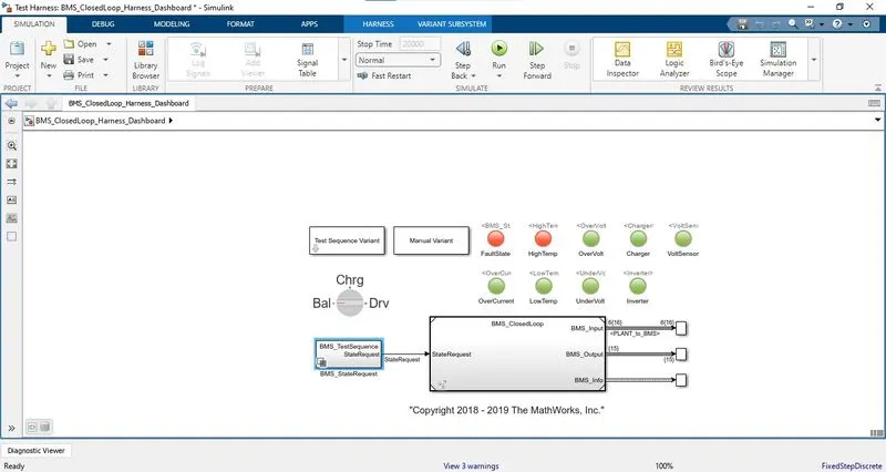
                                                           Figure (18): Harness Dashboard after simulation of test case 2.

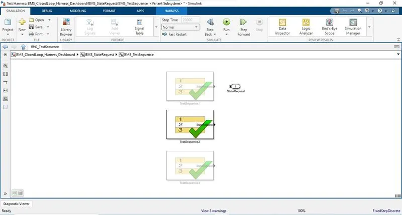
                                                               Figure (19): Test case Selection.

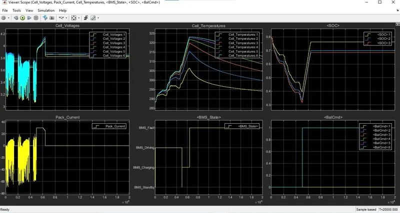
                                          Figure (20): Output of BMS harness after simulation of Test Case 2.

The voltages of the cells in a battery pack will vary according to the current supplied to the cells and the Voltages of the cells are lies between in the range of 3.18V to 3.9V till the time of around 1400 seconds and after 1400 seconds the voltage will be constant for each cells and the constant voltage line will remain till the 2000 seconds. After 2000 seconds the voltage of cells will vary in the range of 3.1V to 3.85V up to the simulation time duration attains above 3800 second and after the voltages will remain constant, that constant voltage of individual cells will remain till above 4500 seconds and after the voltage will vary 3.1V to 3.75V and till 4500 seconds. After 4500 second the voltage will increase gradually to 4.1V till above 6200 second, after that the voltage will decreases to the 3.85V suddenly and the voltage will remains constant till the end of the simulation.

The cell temperatures of battery pack will be different for each individual cell. The cell number six has the highest temperature of 323.2 degrees and cell number one has the lowest cell temperature of 306.4 degrees. The process initializes at 289 degrees and the temperature of the cells gradually increases till the simulation process attains above 6200 seconds and the temperature range is lies between 306 degrees to 323 degrees. After 6200 seconds the temperature graph starts depleting gradually till the end of the simulation. 

The state of charge for the cells initializes the simulation at 80% and the state of charge percent will deplete gradually till 4500 seconds and at 4500 seconds the state of charge is at 35%. After 4500 seconds the state of charge will starts increasing till SOC reaches to 69%, 70% and 76% until the simulation time attains above 6200 seconds and after the state of charge will remains same till the end of the simulation.

The pack current will initializes the simulation process at 0A and the current will increase and decrease in the range between 10A to -70A and the current will be at 0A till the simulation attains 2000 seconds. After 2000 seconds the current will fluctuates up and down in the range between 9A to -65A till the simulation attains to 3900 seconds. After 4200 seconds the current will fluctuates 9A to -60A for 800 seconds and then the current will increases to 30A and it will remains for 1000 seconds. After 6000 seconds the current will depletes to 0A and the current will remains at 0A till the end of the simulation.

The battery management system starts the process at BMS_standby state and it will moves to charging and driving state. The BMS is at driving state till 5000 seconds and after the BMS will goes back to standby state and than charging till 6200 seconds. After 6200 seconds the BMS shows BMS_fault indication due to lack of current and voltage. And the process will stuck at the BMS_fault till the end of the simulation.

The balancing command graph visualizes that, the cell on will remains at 0 from initial state to end of the simulation. The cell six will starts at 0 and it will remains at 0 till 5000 seconds, after it will reaches to 1 and it will remains at 1 till the end of the simulation.

The main reason to show the red flags on the lamp block in the dashboard is due to lack of current and voltage in the cells. With respect to current the voltage will vary, the temperature and SOC will vary with respect to the current and voltage. So the cell temperature reaches very high. Due to lack of voltage and current the BMS will shows the fault in the simulation process.

Test Condition 3:

This condition is only to study the cell charging during the simulation of 20000 seconds. The test harness model does not have any changes and it remains same as shown in figures (21) and (22) for test case selection and dashboard respectively.

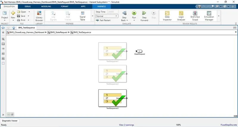
                                                        Figure (21): Test Case 3 Selection

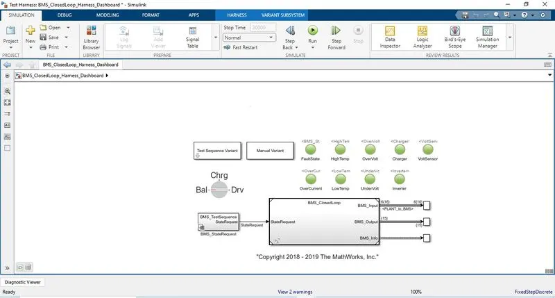
                                           Figure (22): Harness Dashboard Test case 3

The scope results of test case 3 is shown in figure (23).

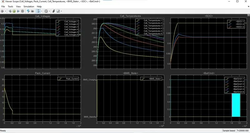
                                            Figure (23): Scope result for Test Case 3

f we observe here that we only given the charging in the model as an input for the 20000 sec.

The voltage in the graph is raises from 4.1V to 4.2V very quick due to CC then after that due to the CV it takes time to charge with CV after that fully charged it gets been constant with 4.1V up to 2000 sec.

If we see the current graph that it raises to 30A in the CC time. After that in the CV time it gets reduced to minimum value and then it gets to 0A due to it reached the fully charged condition. The battery pack current initialize the process at 20A and it depletes gradually 1A at the time range of 2000 seconds. After 2000 seconds the current depletes to 0A, and it will remains at 0A till the end of simulation time.

In cell temperature at CC an CV the temperature raises immediately at CC and increased little slow at CV. When the battery pack get fully charged it start reducing the temperature but it is in the limited ranges only. The Cell Temperature graph starts at 288 degrees and the temperature will increase gradually till the time of around 1200 seconds and the maximum temperature at 1200 seconds is 293 degrees. And we can visualize the slight depletion in temperature till 4000 seconds. After 4000 seconds the temperature is moves like a straight line, all the cells have different temperature ranges. The temperature traces shows the discrepancy in between the highest and lowest temperature cells, due to symmetry in the merged layer in terms of the cell thermal character and behaviour. Cell number six has highest temperature and cell number one has lowest temperature because the cell one has thermal insulation at one end. The active battery managements system will maintains a very less temperature difference between the cells.

In the BMS state the value shown the line in the charging because we using the charging for the entire 20000 sec.

In the SOC graph the values changes from 80% to 100% because it already has the charging value of about 80%. After getting the value to the max charge condition the value remains constant in the battery pack.

In the balancing command the values are plotted based on the values of the cell in the voltages. By changing the values which changed out of range it starts balancing and again it gets off when it reached to limit values. The Battery management system on charging state and Battery command passing signal between 0 to 1.

2. Coulomb counting:

The State of Charge (SoC of a battery cell is required to maintain it's safe operation and lifetime during charge, discharge and storage. However, SoC cannot be measured directly and is estimated from other measurements and known parameters. This leads to errors in the estimated SoC and that means it is not possible to fully exploit the full capability of the cell. The easiest method to calculate the SoC of a battery is by using voltage translation method. This method is not accurate. but helps to approximately and quickly calculate SoC and can be used in devices. There are several limitations in this method and hence more accurate methods are needed like Coulomb counting method, the Fuzzy logic method, the Kalman filter, the RBF Neural network, the Fuzzy Neural network, the Hybrid methods, etc.

The coulomb counting method is also known as the battery current integration method. In this method, a discharging or charging current I(t) is measured and integrated over time to calculate the amount of energy remaining inside the battery. In this method, SoC is taken at the previous time step SoC(t-1) and the amount of energy removed or added at the current time step is subtracted or added from the SoC of the previous time step SoC(t-1) to obtain the amount of energy present in the battery at the present instant. Coulomb counting is a technique used to track the state of charge of a battery pack. It works by integrating the active flowing current (measured in amps) over time to derive the total sum of energy entering or leaving the battery pack. This produces a capacity that is typically measured in Amph-hours. The relation is given as follows:

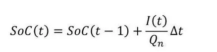
Where,

SoC(t) = estimated State of Charge at time, t.

SoC(t-1) = previous State of Charge at time t-1.

I(t) = Charging or discharging current at time t.

Qn = Battery cell capacity.

`Delta`t = time step between (t-1) and t.

If we want to know the absolute SoC we need to know the starting SoC of the cell, SoC(t-1) as given in the equation. One option is to fully ccharge the cell to known voltage. Charging to maximum cell voltage and SoC can be used as a reset and known point. There are number of sources of error with the coulomb counting method:

i) Starting SoC accuracy.

ii) Current measurement accuracy.

iii) Current integration error.

iv) Uncertainity in battery capacity.

v) timing Error.

Modified Coulomb Counting Method:

To improve the Coulomb counting method, a new technique called modified Coulomb counting method is proposed. The modified Coulomb counting method uses the corrected current to improve the accuracy of estimation. The corrected current is the function of discharging current. There is a quadratic relationship between the corrected current and discharging current of battery. By practice of experimental data, corrected current is calculated by the following form:

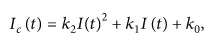
where, k2, k1 and k0 are constant values obtained from the pratice experimental data.

SoC Estimation in Battery Model:

To observe the coulomb counting method, we need to open the SoC_Estimation block of BMS ECU model as shown in figure (24).

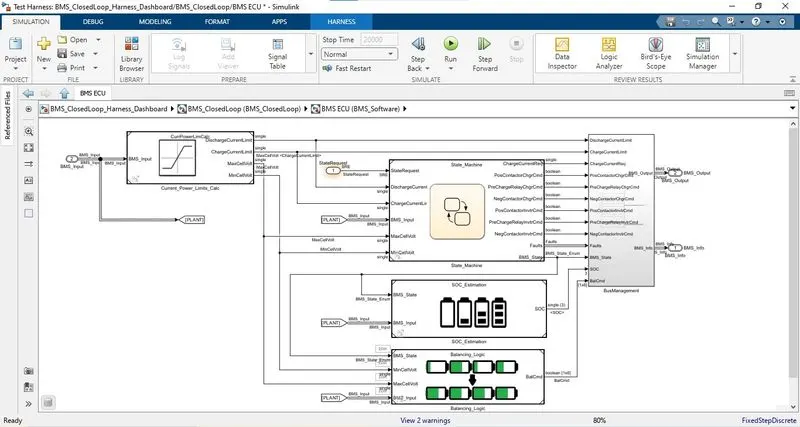
                                       Figure (24): SoC Estimation block for BMS ECU model.

Here, we can see that there are three methods for calculating SoC and these are:

i) Coulomb Counting.

ii) Unscented Kalman Filter.

iii) Extended Kalman Filter.

Figure (25) shows the three methods of SoC estimation in the model.

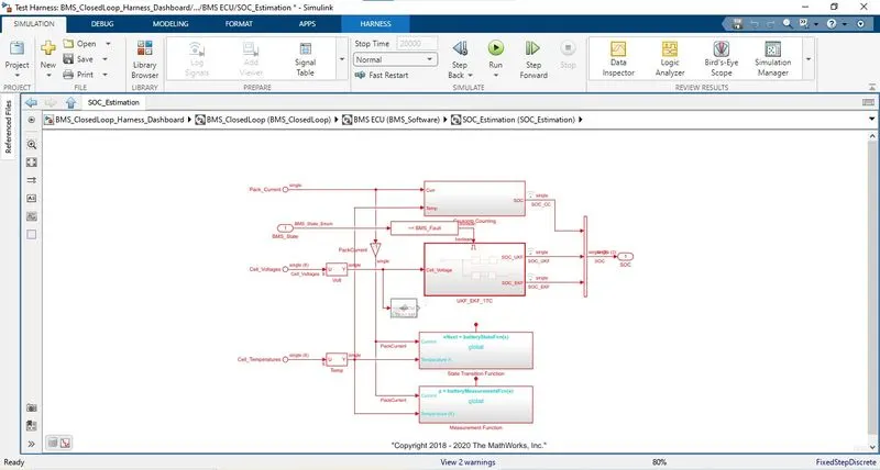
                                      Figure (25): SoC Estimation Methods.

By opening the coulomb counting method, as shown in figure (26), we get to see the gain, 1-D look up table, product and discrete time integrator block.

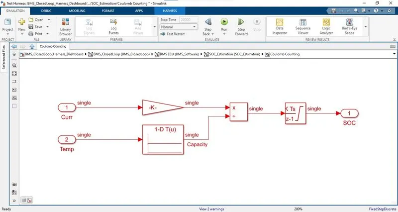
                                                 Figure (26): Coulomb counting method Block.

The discharge current from the battery is given to a gain having a value of 1/3600 to convert A to Ah as shown in figure (27).

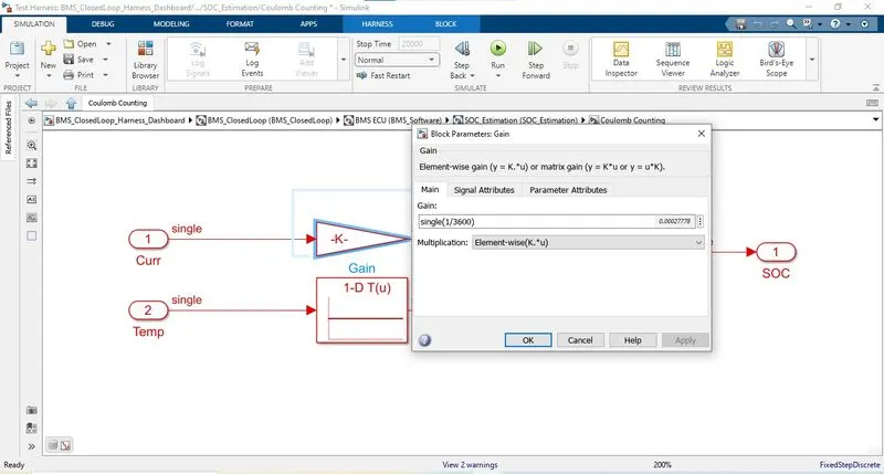
                                    Figure (27): Gain Value

Two inputs come into the system: current and temperature of the pack. Current, as said above is converted to capacity (Ah). then based on the temperature the pack capacity is estimated. This estimated capacity is divided by the discharge capacity and integrated over time which gives the SoC at any given instant.