Week 7 State of charge estimation
The simulation of the 3 test cases from harness dashboard is as follows:-
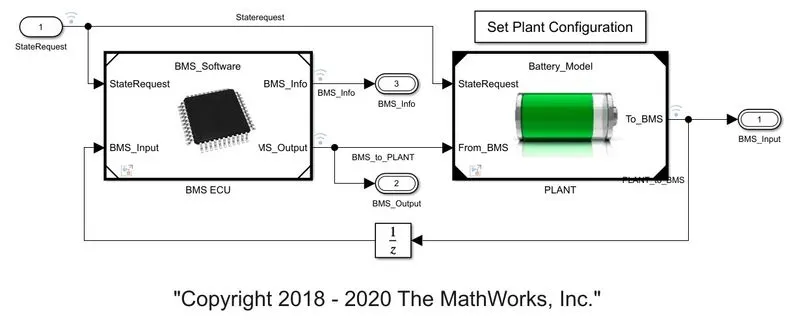
FIG 1 : BMS SYSTEM
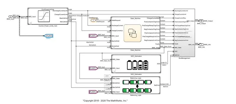
FIG 2 : BMS ECU
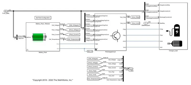
FIG 3 : BATTERY MODEL
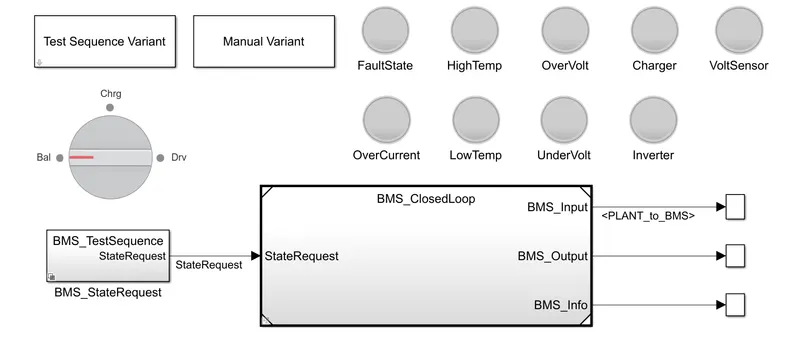
FIG 4 : BMS CLOSED LOOP HARNESS DASHBOARD
Here we double click on test sequence variant and test for 3 test sequences as follows:
(1) Test Sequence 01:
The simulation is run for 20000 seconds as we can see in the simulation results plot, in which the first 3000 seconds is the discharge or the driving mode then the next 1000 seconds are in balancing or standby mode then for 5000 seconds in charging and balancing mode and afterwards the in standby or balancing mode.
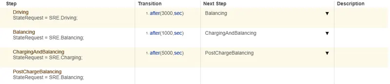
FIG 5 : SHOWING STEPS, TRANSITION AND THE NEXT STEP
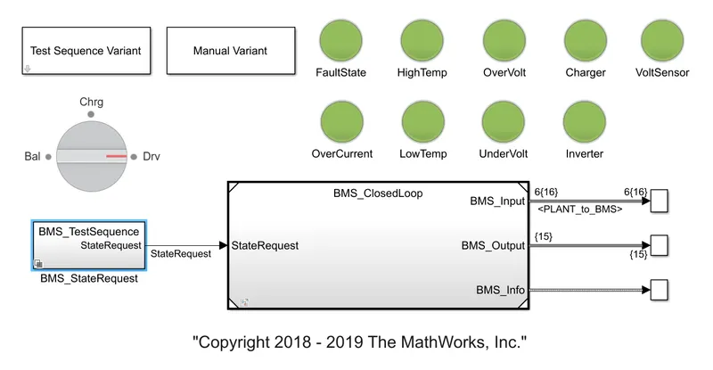
FIG 6 : BMS CLOSED LOOP HARNESS AFTER RUNNING TEST SEQUENCE 1
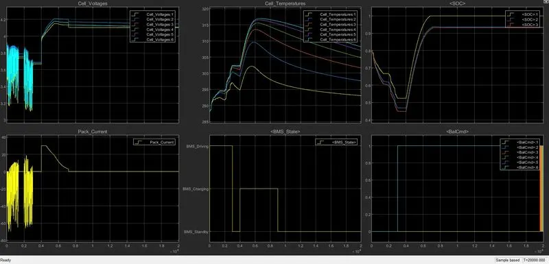
FIG 7 : SIMULATION RESULTS OF TEST SEQUENCE 1
- The first plot with Cell_Voltages displays the voltages of all 6 cells connected in the series. While the first 3000 seconds the voltage of the cells drops as the battery is discharging and during the standby period the voltage stabilizes as the cell balancing gets activated and even due to cell inherit behaviour. Then while charging the cell voltage increases and while the cell balancing the voltage stabilizes.
- The second plot with Pack_Current represents the current drawn and given to the battery while charging and discharging. It is also seen that while charging, first the current remains constant, and then it drops its charges in constant voltage mode.
- The third plots the cell temperature of all individual cells and we can see then while charging and discharging the cell temperature increases.
- The fourth plot shows the input state as per the given state input.
- The fifth plot shows the state of charge of the entire pack by 3 different methods of calculation. The soc curve decreases as we discharge the battery and increases while charging.
- The sixth plot shows the cell balancing command for all six cells. The 1st cell is having the lowest voltage does not need balancing thus we can see that all the other cell's signal have a magnitude of 1 whereas the 1st cell signal is at zero magnitudes.
(2) Test Sequence 02:
The simulation is to run for 20000 seconds in which the first 5000 seconds is the discharge or the driving mode then the rest of the time is set to charge the battery.

FIG 8 : TEST SEQUENCE 2 TRANSITIONS
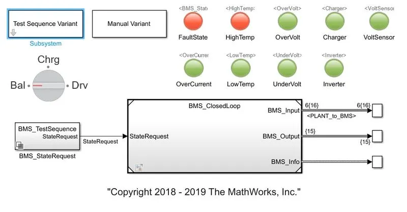
FIG 9 : BMS CLOSED LOOP HARNESS DASHBOARD AFTER RUNNING TEST SEQUENCE 2
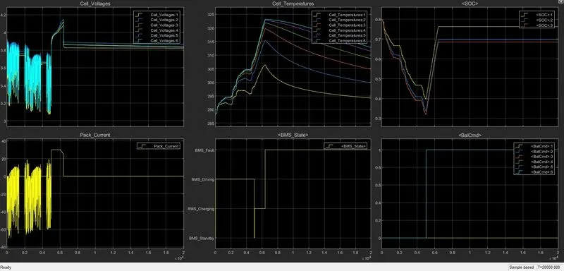
FIG 10 : SIMULATION RESULTS OF TEST SEQUENCE 2
- The first plot with Cell_Voltages displays the voltages of all 6 cells connected in the series. While the first 5000 seconds the voltage of the cells drops as the battery is discharging and then while charging the cell voltage increases and while the cell balancing the voltage stabilizes.
- The second plot with Pack_Current represents the current drawn and given to the battery while charging and discharging. It is also seen that while charging, first the current remains constant, and then it drops its charges in constant voltage mode.
- The third plots the cell temperature of all individual cells and we can see then while charging and discharging the cell temperature increases, at about 6000 seconds the cell temperature of the 6th cell increases to about 323.15 Kelvin, and the battery is sent to fault state.
- The fourth plot shows the input state as per the given state input until the fault occurs at about 6000 seconds.
- The fifth plot shows the state of charge of the entire pack by 3 different methods of calculation. The soc curve decreases as we discharge the battery and increases while charging. The battery is charged up to 70-75% and stops charging once the fault occurs.
- The sixth plot shows the cell balancing command for all six cells. The 1st cell is having the lowest voltage does not need balancing thus we can see that all the other cell's signal have a magnitude of 1 whereas the 1st cell signal is at zero magnitudes. The cell balancing starts when the battery starts to charge and at the onset of the fault the battery charging is stopped but the balancing happens.
(3) Test Sequence 03:
The simulation is run for 20000 seconds in which the first 10000 seconds is the discharge or the driving mode then the rest of the time is set to charge the battery.

FIG 11 : TEST SEQUENCE 3 STATE TRANSITIONS
FIG 12 : BMS CLOSED LOOP HARNESS DASHBOARD AFTER RUNNING TEST SEQUENCE 3
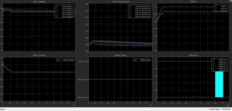
FIG 13 : SIMULATION RESULTS OF TEST SEQUENCE 3
- The first plot with Cell_Voltages displays the voltages of all 6 cells connected in the series. The cell voltage keeps on dropping as the battery keeps on discharging up to zero state of charge and the simulation is stopped.
- The second plot with Pack_Current represents the current drawn and given to the battery while charging and discharging. Here we can see that battery repeats the charging and discharging pattern as explained above in the charging and discharging load.
- The third plots the cell temperature of all individual cells and we can see then while charging and discharging the cell temperature increases.
- The fourth plot shows the input state as per the given state input, the simulation only runs in discharging mode and when the SOC reaches zero the simulation is stopped at about 8692 seconds.
- The fifth plot shows the state of charge of the entire pack by 3 different methods of calculation. The soc curve decreases as we discharge the battery and increases while charging. Here the battery keeps on discharging as the regenerative charging is very less.
- The sixth plot shows the cell balancing command for all six cells. The cell balancing does not take place as the simulation runs only in a driving state.
(2) Coulomb counting:
Coulomb counting is a technique used to track the state of charge of a battery pack. It works by integrating the active flowing current (measured in amps) over time to derive the total sum of energy entering or leaving the battery pack. This produces a capacity that is typically measured in Amp-hours.
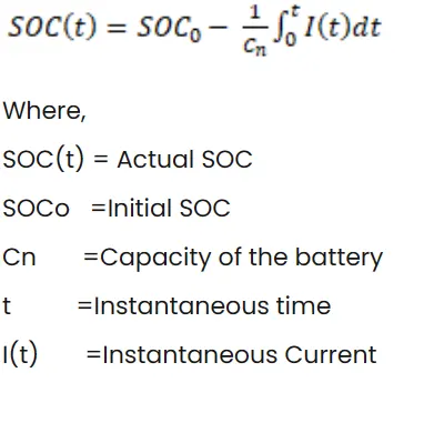
The Coulomb counting method measures the discharging current of a battery and integrates the discharging current over time in order to estimate SOC. It is done to estimate the SOC(t), which is estimated from the discharging current, I(t), and previously estimated SOC values, SOC(t-1). SOC is calculated by the following equation:
Implementation of coulomb counting for SOC estimation in the BMS:
To compute the SOC of battery, insert a plant block into the model.
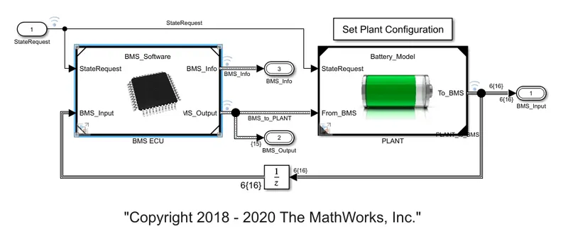
BMS algorithm models , protects , reports the measurement from battery pack.
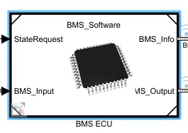
When we click on BMS ECU block we get,
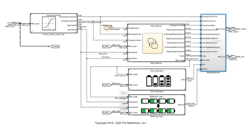
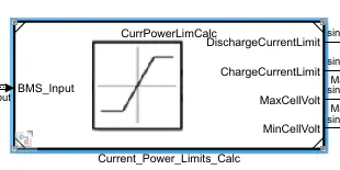
By clicking on the current power limit calc block , we get the below block diagram.
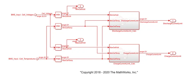
Here the cell voltage and cell temperature is used to decide maximum allowable charging and discharging current limits.when cell is at lowest SOC , its voltage is low,and thus it is important to prevent cell from delivering large amount of current because it wil cause large voltage drop that could be potential below the cut off voltage specify by the cell manufacture.
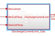
Click on dischargecurrentlimit calc block, we get the following block diagram shown below,
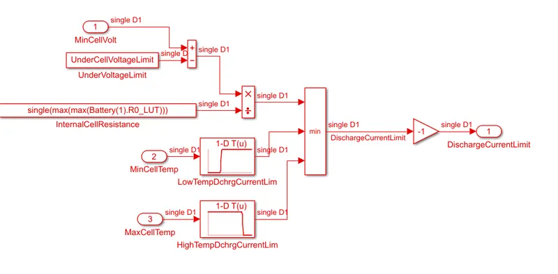
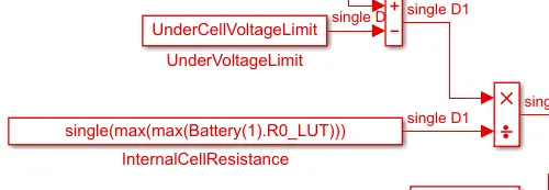
Here by comparing the minimum cell voltage in the module against this lowest threshold voltage and then divided by maximum internal cell resistance value, , we can compute the voltage based threshold.
It is also important to limit the current delivery and current intake when temperature is too high or too low. Using the lockup table with rising and falling s shape profile, we can specify current threshold based temperature and thus can modulate allowable current delivery. It is recommended to avoid low and high temperature during discharging and low temperature during charging.
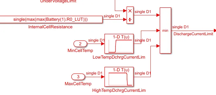
Then the above two threshold are then compared and minimum of this two becomes the current limit. Knowing how much longer we can able to drive our car before we had to stop for recharge depends on the accurate estimation of battery SOC. In battery system, we do not measure SOC directly, we actually measure something else and then relate it with SOC.
3 methods are used for SOC estimation, but coulomb counting is mostly used.
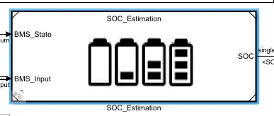
click on soc estimation block , we get,
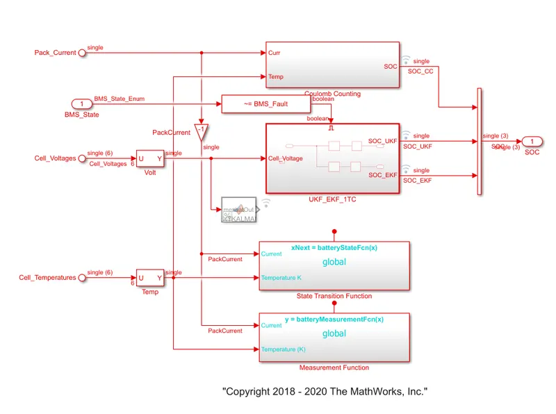
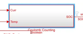
By clicking on coulomb counting block , we get the below block diagram
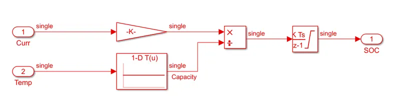
In this coulomb counting method, the entering and leaving currents of the cell are integrated to track the safe chargable time. Here the two input signals current and temperature are taken the curent signal goes to gain block and the temperature signal goes to current look up table, then as seen, signals are multiplied and divided as shown and then output is given to discrete time integrator to track the safe chargable time and then SOC is estimated.
Advantage of coulomb counting method is its simplicity and low computational cost.
The drawback of coulomb counting method is accumulation of current sensor error and inability to recover from wrong initial condition because of lack of feedback from voltage measurement.