Week 7 State of charge estimation

week 7 state of charge estimation

Aim:

• To simulate the 3test cases from harness dashboard and write a detailed report on the results from the given MATLAB file.
• To define coulomb counting by referring to the above model and explain how BMS implements Columb counting for SOC estimation.

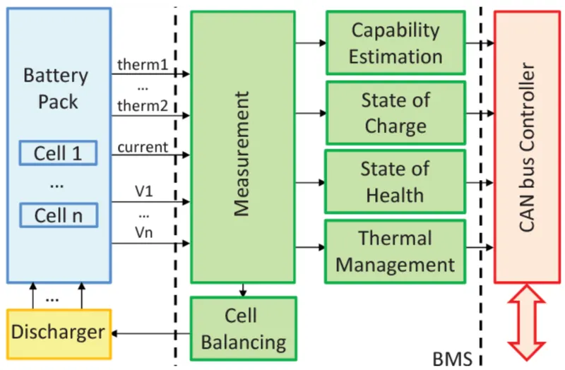
Battery management system (BMS): BMS is used to control the battery pack electronics, which includes electrical and digital data. It is an embedded system, which is a combination of hardware and software. The main functions of a BMS are to protect batteries from operating outside its safe operating area, monitoring its state, calculating the secondary data, reporting that data, controlling its environment, authenticating it balancing it.

BMS working flow chart

The given MATLAB project file is used as a reference design to get started with designing BMS with MATLAB and Simulink.

This project includes Simulink models for BMS algorithms such as

• State of charge estimation using extended Kalman filter, unscented Kalman filter.
• Passive battery cell balancing.
• State machine for pre-charging and contactor management.
• Fault management - over/under voltage, over current, over temperature etc.
• Charge and discharge current limit calculations.

To design and test these algorithms, the project also includes files for

• Li-ion battery cell parameter estimation.
• Battery pack with 6 cells in series and 96 cells in series.
• Simulink test files with test cases to test state machine logic
• Linking requirements to models.

BMS closed loop harness dashboard model file

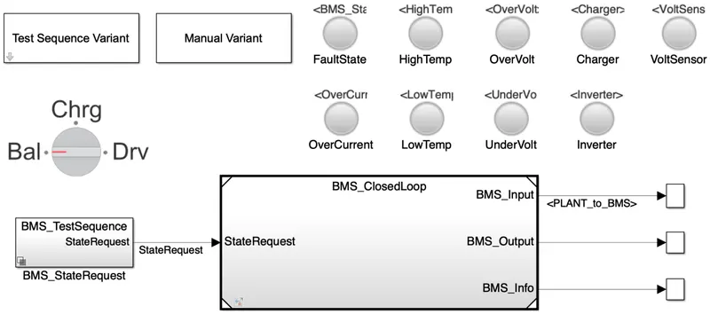
It has three different test conditions.

• Manual variant
• BMS state request subsystem to provide the state request commands.
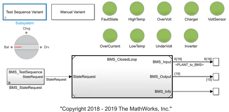
• The indicating lamps are there to show any faults state high temperature overvoltage charger voltage sensor overcurrent low temperature under voltage inverter state of battery.
• The green light tells us that all states are OK and battery is good to charge and discharge and red indication will indicate the fault state.
• The rotating switch for manual variant to change the position during simulation run time

1^st test

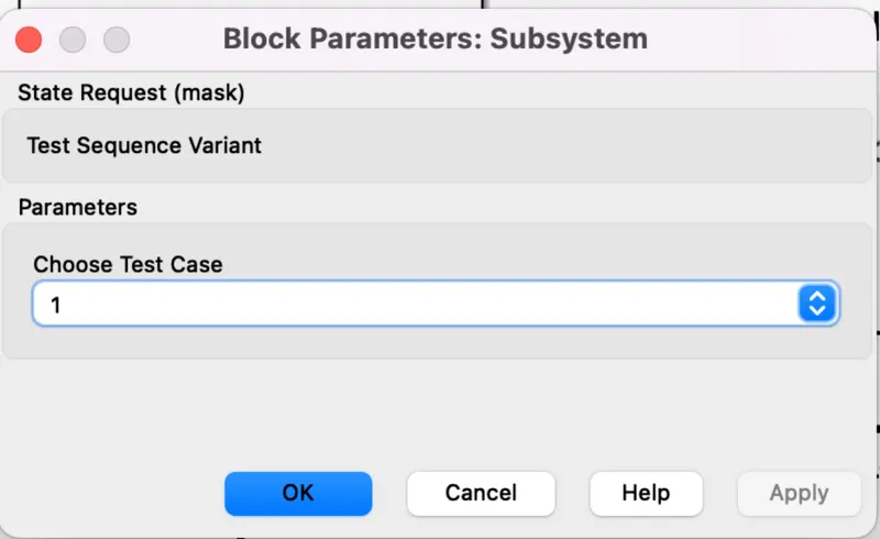
Here test case 1 is selected as shown in the below figure

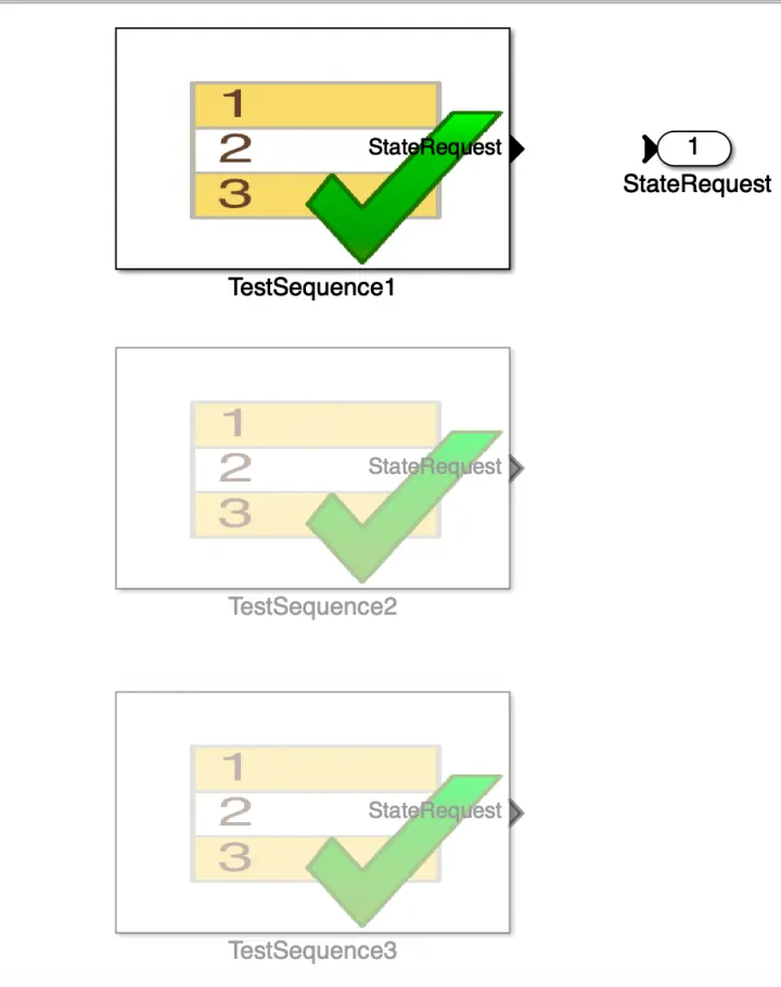
The flow chart for this test condition is as follows

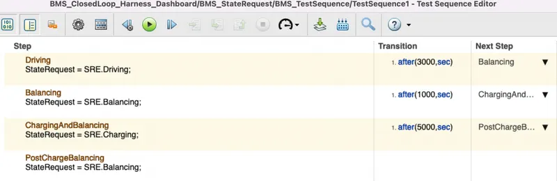
• Here from the above fig, it tells about the test sequence
• For driving is done for first 3000 secs
• Then after driving the balancing of cell comes for the next 1000 secs.
• So, after the balancing charging and balancing comes for next 5000 secs.
• But in post charging balancing it occurs after the 9000secs till 20000sec.

Results for case 1

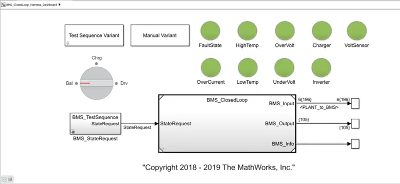
• Here we can see that all the indicators are green.
• So, we can see no errors and we check the plot for this model and is below.
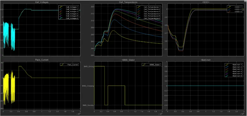
• From the above plot we can see the vehicle is initially in a driving state and charging was done by 90%.
• So, after charging it reaches standby mode. It can be seen in the BMS state plot. Battery temperature increases in driving and charging.
• The battery voltage was increased to 4.2V while charging.
• The current plot shows the value of current supplied to the vehicle while driving.
• Hence SOC decreased up to 50% driving conditions and it was increased while charging.

Test Case 2:

In the test sequence choose the test case parameters to 2

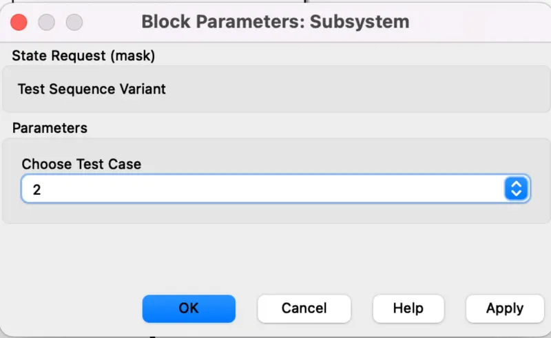
Here we changed the test sequence number from the subsystem to 2

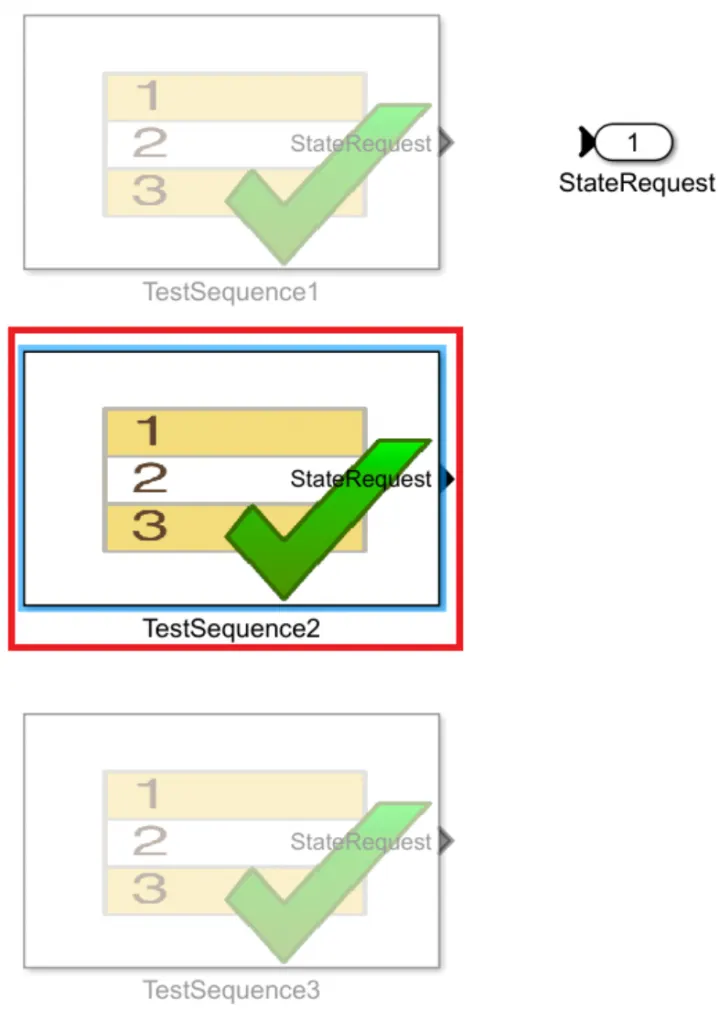
The flow chart for this test is as follows

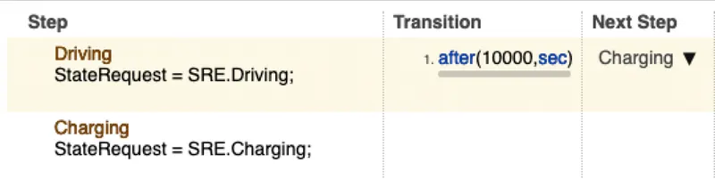
Here all the details of the test will be performed in the simulation.

So, the driving stage is from 0 to 5000secs and then charging.

Results

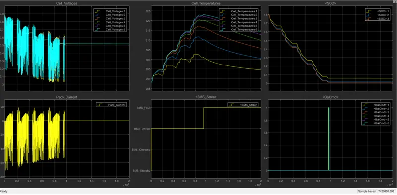
• Here in driving cycle mode i.e. 0-10000 sec the cell voltage varies from 3.9 to 3.05V which is the cutoff voltage of a cell and the entire cell is drained upto 8692 secs.
• So, the cell temperature changes from 288k to 322k.
• The SOC decreased from 80% to 0%.
• Some in the charging mode i.e. 10000 to 20000 sec the cell got drained earlier before it reached this mode.

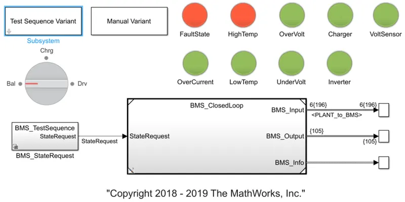
The result shows that there is a fault condition in the vehicle. The dashboard on the model depicts the same with a red color indication.

Test Case 3

Change the parameter in the test sequence to 3

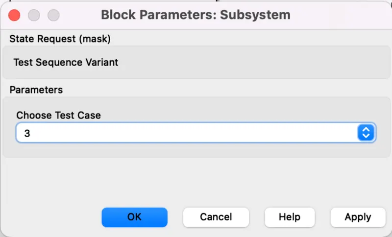
Here we selected test case 3

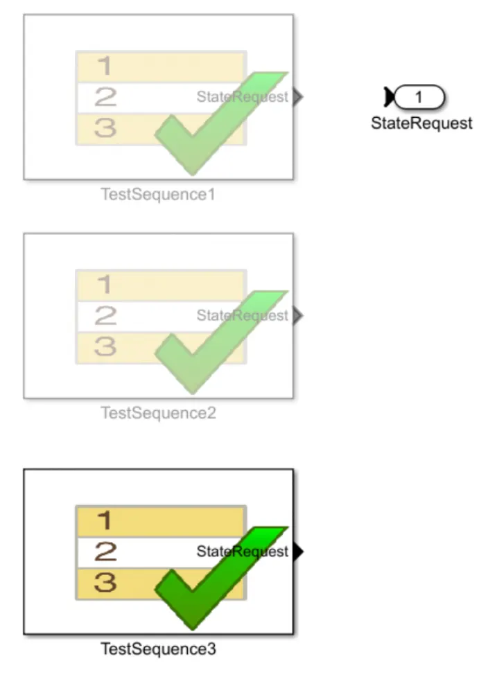
Here the flow chart for this test condition is as follows

In this flow chart we can only see one BMS state that is charging. So, from 0 seconds till 20000 secs only charging is done.

Now let us simulate the second test condition and look at the results

Results

The dashboard shows no error, since all LEDs are green in color as shown below.

The scope results for the second test are shown below

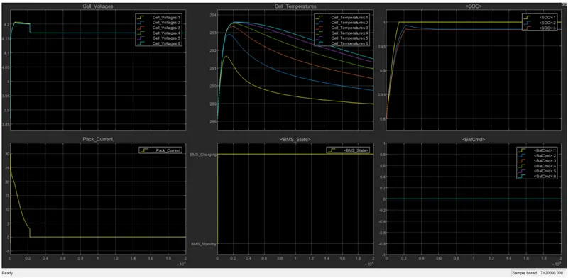
• Here we can see that at the beginning of the simulation battery is at 80% SOC. Now the charging starts once the simulation begins and by 1800 secs the battery pack is fully charged and the SOC reaches 100%
• In the cell voltages plot we can see that the maximum voltage is reached during the charging and once the SOC is at 100% the voltage starts decreasing and attains a stable value between 4.1V and 4.15V.
• The maximum cell temperature of 292.5k is reached when the battery is fully charged and after that the temperature starts reducing.
• In the pack current plot, we can see that the highest transient current reached is 30A and it starts decreasing as the charging progresses.

STATE OF CHARGE ESTIMATION

COULOMB COUNTING

The State of Charge (SOC) estimation is done in this model by using a method called Coulomb Counting. This particular method measures the discharging current of a battery and integrates the discharging current over time in order to estimate SOC. Soc is calculated by the following equation.

SOC(t)= SOC(t-1) +((I(t))/Q_n)t

The accuracy of Coulomb counting method depends on temperature, battery history, discharge current and life cycle. The Coulomb counting method accumulates error over the period of time and hence it is not preferred method for simulations taking longer duration of time. This error is caused due to the fact that the exact values of cell total capacity, current experienced by the cell , coulombic efficiency and the amount of current drawn to power the electronic circuitry that monitors its performance is not known. The Coulomb counting block diagram used in this model is shown below,

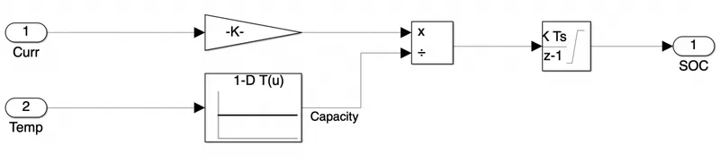
Here we can see there are two inputs, one is current and the other is temperature.

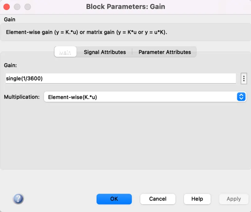
The current input is connected to the gain block, whose value is as shown below,

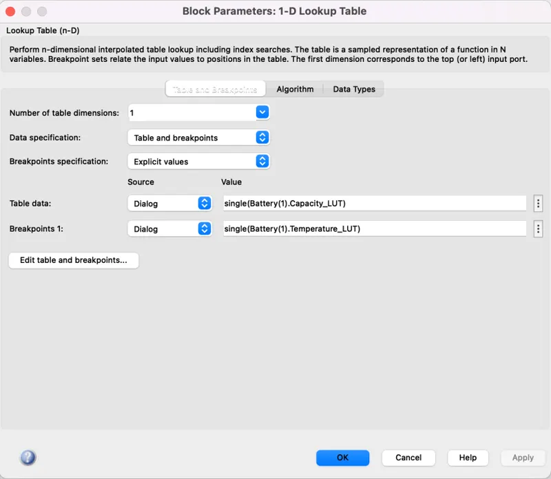
The temperature input is connected to a lookup table containing capacity values at each temperature.

This lookup table is shown below with its values

Now the output from the gain block is divided by the output from the lookup table block.

And then it's connected to a discrete time integrator block.

This block and its parameters are shown below,

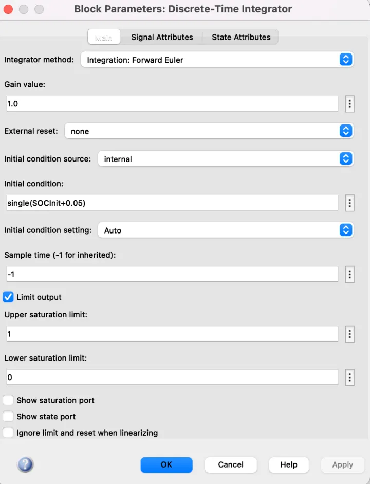
The block will accumulate the SOC value over time.

This is how the BMS implements coulomb counting for SOC estimation.

Conclusion

The 3 test cases from harness dashboard in the given MATLAB file have been simulated and the results have been explained successfully.

Also, the implementation of coulomb counting by the BMS for SOC estimation has been explained.