Week 7 - Simulation of a 1D Supersonic nozzle flow simulation using Macormack Method

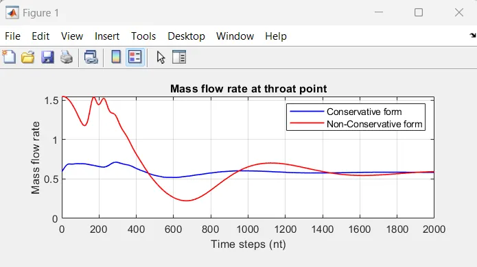
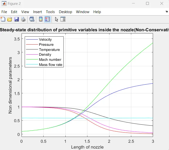
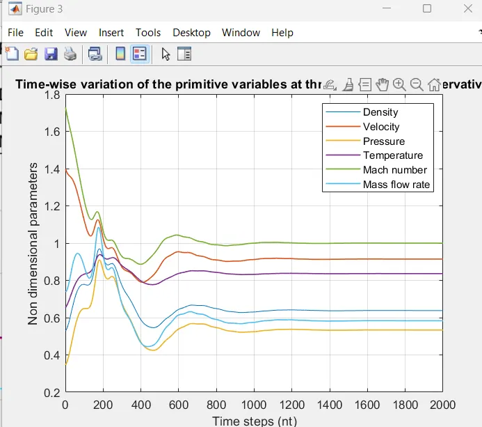
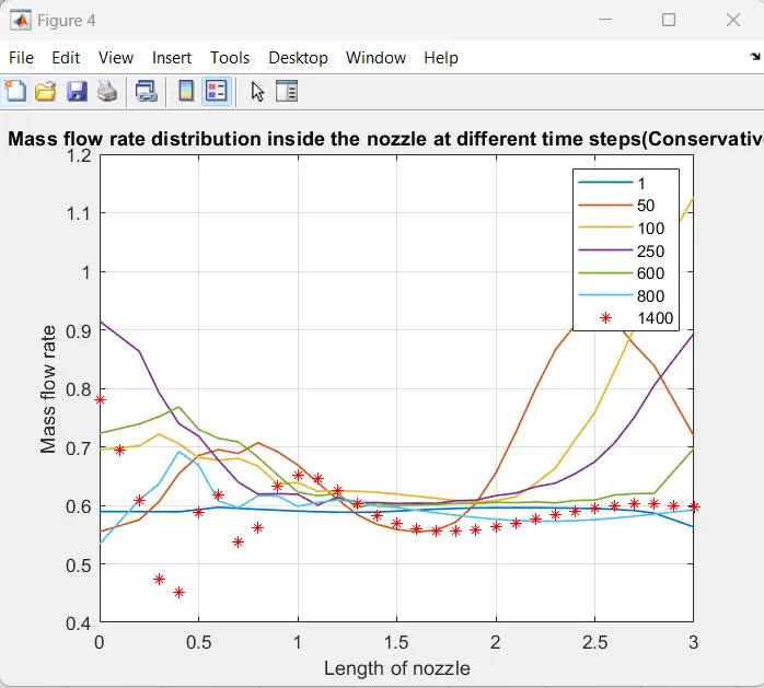
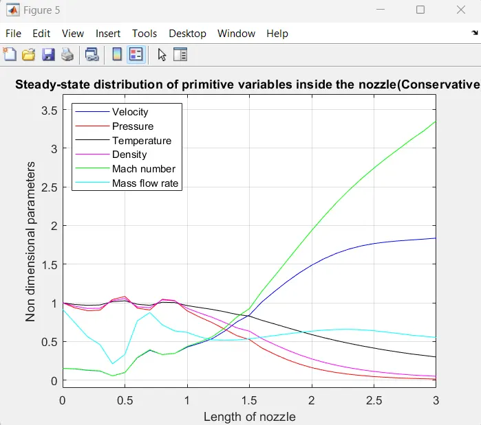
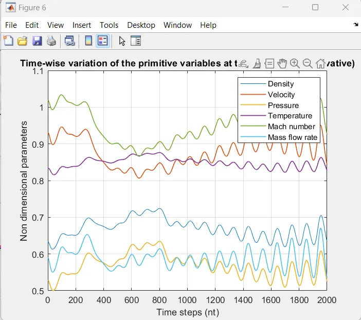
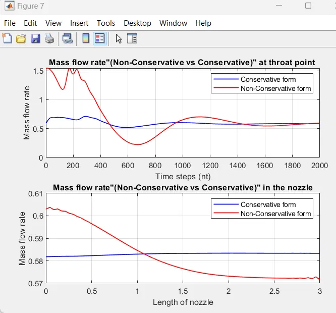
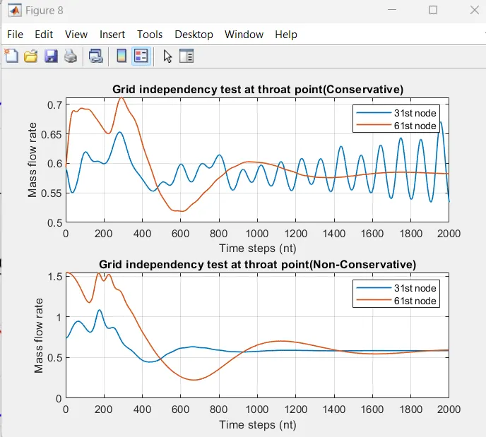
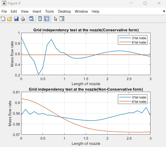
Matlab code: close all clear all clc %Week 7 - Simulation of a 1D Supersonic nozzle flow simulation using macormack method L = 3; % Length of nozzle n = [31 71]; % Grid points on z and xory axis, % taken from anderson book 31 node nuber represents throat nt = 1:2000; %time steps cfl = 0.2; %CFL number for i = 1:length(n) %as x axis taken for length. iteration is done for each grid point on z axis x = linspace(0, L, n(i)); % Calling non-conservative and conservative functions [mfr_nc, mfr_throat_nc] = non_conservative(L, n(i), nt, cfl); [mfr_c, mfr_throat_c] = conservative(L, n(i), nt, cfl); % Plotting figure(1) subplot(2, 1, 1) plot(nt, mfr_throat_c, 'b', nt, mfr_throat_nc, 'r', 'linewidth', 1) xlabel('Time steps (nt)') ylabel('Mass flow rate') legend('Conservative form', 'Non-Conservative form') title('Mass flow rate at throat point') grid on figure(7) subplot(2,1,1) plot(nt,mfr_throat_c,'b',nt,mfr_throat_nc,'r','linewidth',1) xlabel('Time steps (nt)') ylabel('Mass flow rate') legend('Conservative form','Non-Conservative form') title('Mass flow rate"(Non-Conservative vs Conservative)" at throat point ') grid on subplot (2,1,2) plot(x,mfr_c,'b',x,mfr_nc,'r','linewidth',1) xlabel('Length of nozzle') ylabel('Mass flow rate') legend('Conservative form','Non-Conservative form') title('Mass flow rate"(Non-Conservative vs Conservative)" in the nozzle') grid on figure(8) subplot (2,1,1) plot(nt,mfr_throat_c,'linewidth',1) hold on xlabel('Time steps (nt)') ylabel('Mass flow rate') legend('31st node','61st node') title('Grid independency test at throat point(Conservative)') grid on subplot (2,1,2) plot(nt,mfr_throat_nc,'linewidth',1) hold on xlabel('Time steps (nt)') ylabel('Mass flow rate') legend('31st node','61st node') title('Grid independency test at throat point(Non-Conservative)') grid on figure(9) subplot (2,1,1) plot(x,mfr_c,'linewidth',1) hold on xlabel('Length of nozzle') ylabel('Mass flow rate') legend('31st node','61st node') title('Grid independency test at the nozzle(Conservative form)') grid on subplot (2,1,2) plot(x,mfr_nc,'linewidth',1) hold on xlabel('Length of nozzle') ylabel('Mass flow rate') legend('31st node','61st node') title('Grid independency test at the nozzle(Non-Conservative form)') grid on end function codes: %FUNCTION CODE FOR NON CONSERVATIVE FORM function [mfr_nc,mfr_throat_nc]=non_conservative(L,n,nt,cfl) x=linspace(0,L,n); dx=x(2)-x(1); % initial conditions rho, a, v, T, mfr, M, p rho = 1-0.3146*x; %density (rho) T= 1-0.2314*x; %temperature (T) v=(0.1+1.09*x).*T.^0.5; %velocity (v) %area a= 1+2.2*(x-1.5).^2; %area (a) M= v./(T.^0.5); %mack number mfr = rho.*a.*v; %mass flow rate p=rho.*T; %pressure (p) g = 1.4;%gamma value for z=1:31 u=(T(z))^(1/2); dt(z) = cfl*dx/(u + v(z)); end dt=min(dt); for i = 1:length(nt) %storing initial values rho_old = rho; T_old = T; v_old = v; for j=2:n-1 %predictor step drho_dx = (rho(j+1)-rho(j))/dx; dv_dx = (v(j+1)-v(j))/dx; dT_dx = (T(j+1)-T(j))/dx; da_dx = (log(a(j+1))-log(a(j)))/dx; % continuity equation drho_dt_p(j) = -rho(j)*dv_dx - rho(j)*v(j)*da_dx - v(j)*drho_dx; % momentum equation dv_dt_p(j) = -v(j)*dv_dx - (1/g)*(dT_dx + (T(j)/rho(j))*drho_dx); % energy equation dT_dt_p(j) = -v(j)*dT_dx - (g-1)*T(j)*(dv_dx + v(j)*da_dx); %updating primitives v(j) = v_old(j) + dv_dt_p(j)*dt; rho(j) = rho_old(j) + drho_dt_p(j)*dt; T(j) = T_old(j) + dT_dt_p(j)*dt; %corrector step drho_dx = (rho(j)-rho(j-1))/dx; dv_dx = (v(j)-v(j-1))/dx; dT_dx = (T(j)-T(j-1))/dx; da_dx = (log(a(j))-log(a(j-1)))/dx; % continuity equation drho_dt_c(j) = -rho(j)*dv_dx - rho(j)*v(j)*da_dx - v(j)*drho_dx; % momentum equation dv_dt_c(j) = -v(j)*dv_dx - (1/g)*(dT_dx + (T(j)/rho(j))*drho_dx); % energy equation dT_dt_c(j) = -v(j)*dT_dx - (g-1)*T(j)*(dv_dx + v(j)*da_dx); end %average time derivatives drho_dt_avg = 0.5*(drho_dt_p + drho_dt_c); dv_dt_avg = 0.5*(dv_dt_p + dv_dt_c); dT_dt_avg = 0.5*(dT_dt_p + dT_dt_c); %final corected values for k = 2:n-1 rho(k) = rho_old(k) + drho_dt_avg(k)*dt; v(k) = v_old(k) + dv_dt_avg(k)*dt; T(k) = T_old(k) + dT_dt_avg(k)*dt; end %entry boundary conditions v(1) = 2*v(2)-v(3); %exit boundary conditions v(n) = 2*v(n-1)-v(n-2); rho(n) = 2*rho(n-1)-rho(n-2); T(n) = 2*T(n-1)-T(n-2); %Final update of primitives p = rho.*T; M= v./T.^0.5; error(k) = abs(v(k)-v(k-1)); mfr= rho.*a.*v; %to find values at throat point T_throat(i) = T(16); rho_throat(i) = rho(16); v_throat(i) = v(16); M_throat(i) = M(16); p_throat(i) = p(16); error_throat(i)=error(16); mfr_throat(i)=mfr(16); if n==31 for ii=[1:50:201 700] if ii==i figure(1) plot(x,mfr,'linewidth',1) hold on title ('Mass flow rate inside the nozzle at different time steps(Non-Conservative)') xlabel('Length of nozzle') ylabel('Mass flow rate') elseif i==1400 plot(x,mfr,'*r') legend('1','50','100','250','600','800','1400') grid on end end end end if n==31 figure(2) plot(x,v,'b',x,p,'r',x,T,'k',x,rho,'m',x,M,'g',x,mfr,'c') ylim([-0.1 3.7]) title (sprintf('Time step = %d',i)) xlabel('Length of nozzle') ylabel('Non dimensional parameters') legend('Velocity','Pressure','Temperature','Density','Mach number','Mass flow rate','location','northwest') title('Steady-state distribution of primitive variables inside the nozzle(Non-Conservative)') grid on figure (3) plot(nt,rho_throat) hold on plot(nt,v_throat,'linewidth',1) plot(nt,p_throat,'linewidth',1) plot(nt,T_throat,'linewidth',1) plot(nt,M_throat,'linewidth',1) plot(nt,mfr_throat,'linewidth',1) xlabel('Time steps (nt)') ylabel('Non dimensional parameters') legend('Density','Velocity','Pressure','Temperature','Mach number','Mass flow rate') title('Time-wise variation of the primitive variables at throat point(Non-Conservative)') grid on end mfr_nc=mfr; mfr_throat_nc=mfr_throat; end %FUNCTION CODE FOR CONSERVATIVE FORM function [mfr_c,mfr_throat_c]=conservative(L,n,nt,cfl) x=linspace(0,L,n); dx=x(2)-x(1); % initial conditions rho, a, v, T, M, mfr, p for ii=1:length(x) if (x(ii)<=0.5) rho(ii) = 1; T(ii) = 1; elseif (x(ii)>0.5) & (x(ii)<=1.5) rho(ii) = 1-0.366*(x(ii)-0.5); T(ii)= 1-0.167*(x(ii)-0.5); elseif (x(ii)>1.5) & (x(ii)<=3.5) rho(ii) = 0.634-0.3879*(x(ii)-1.5); T(ii)= 0.833-0.3507*(x(ii)-1.5); end end a= 1+2.2*(x-1.5).^2; %area g = 1.4; %gamma value % solution vectors u1, u2, u3 u1 = rho.*a; u2 = 0.59*ones(1,n); v=u2./u1; u3 = u1.*((T./(g-1))+(g/2).*v.^2); M= v./(T.^0.5); mfr = rho.*a.*v; %mass flow rate p=rho.*T; %pressure for z=1:31 u=(T(z))^(1/2); dt(z) = cfl*dx/(u + v(z)); end dt=min(dt); for i = 1:length(nt) %storing initial values u1_old = u1; u2_old = u2; u3_old = u3; for j=2:n-1 %flux vectors f1 = u2; f2 = ((u2.^2)./u1)+((g-1)/g)*(u3-((g/2)*(u2.^2)./u1)); f3 = ((g.*u2.*u3)./u1) - ((g*(g-1)/2)*(u2.^3)./(u1.^2)); %source term j1 = (1/g)*rho(j)*T(j)*((a(j+1)-a(j))/dx); %predictor step %continuity equation du1_dt_p(j)= -(f1(j+1)-f1(j))/dx; %momentum equation du2_dt_p(j)= -(f2(j+1)-f2(j))/dx + j1; %energy equation du3_dt_p(j)= -(f3(j+1)-f3(j))/dx; %updating solution vectors u1(j) = u1_old(j) + du1_dt_p(j)*dt; u2(j) = u2_old(j) + du2_dt_p(j)*dt; u3(j) = u3_old(j) + du3_dt_p(j)*dt; %updating primitives rho=u1./a; T=(g-1).*(u3./u1-(g/2).*(u2./u1).^2); %updating flux terms f1=u2; f2=u2.^2./u1+((g-1)/g).*(u3-(g/2)*u2.^2./u1); f3=g.*u2.*u3./u1-0.5*g*(g-1).*u2.^3./u1.^2; %source term for corrector step j2 = (1/g)*(rho(j)*T(j)*(a(j)-a(j-1))/dx); %corrector step %continuity equation du1_dt_c(j) = -(f1(j)-f1(j-1))/dx; %momentum equation du2_dt_c(j) = -(f2(j)-f2(j-1))/dx + j2; %energy equation du3_dt_c(j) = -(f3(j)-f3(j-1))/dx; end %average time derivatives du1_dt_avg = 0.5*(du1_dt_p + du1_dt_c); du2_dt_avg = 0.5*(du2_dt_p + du2_dt_c); du3_dt_avg = 0.5*(du3_dt_p + du3_dt_c); %final corected values for k = 2:n-1 u1(k) = u1_old(k) + du1_dt_avg(k)*dt; u2(k) = u2_old(k) + du2_dt_avg(k)*dt; u3(k) = u3_old(k) + du3_dt_avg(k)*dt; end %entry boundary conditions u1(1) = a(1); u2(1) = 2*u2(2)-u2(3); u3(1) = u1(1)*(T(1)/(g-1) + (g*(u2(1)/u1(1))^2)/2); %exit boundary conditions u1(n) = 2*u1(n-1)-u1(n-2); u2(n) = 2*u2(n-1)-u2(n-2); u3(n) = 2*u3(n-1)-u3(n-2); %Final update of primitives rho = u1./a; v = u2./u1; T=(g-1).*(u3./u1-(g/2).*(u2./u1).^2); p = rho.*T; M= v./T.^0.5; error(k) = abs(v(k)-v(k-1)); mfr= u2; %to find values at throat point T_throat(i) = T(16); rho_throat(i) = rho(16); v_throat(i) = v(16); M_throat(i) = M(16); p_throat(i) = p(16); error_throat(i)=error(16); mfr_throat(i)=mfr(16); if n==31 for ii=[1:50:201 700] if ii==i figure(4) plot(x,mfr,'linewidth',1) hold on title ('Mass flow rate distribution inside the nozzle at different time steps(Conservative) ') xlabel('Length of nozzle') ylabel('Mass flow rate') elseif i==1400 plot(x,mfr,'*r') legend('1','50','100','250','600','800','1400') grid on end end end end if n==31 figure(5) plot(x,v,'b',x,p,'r',x,T,'k',x,rho,'m',x,M,'g',x,mfr,'c') ylim([-0.1 3.7]) title (sprintf('Time step = %d',i)) xlabel('Length of nozzle') ylabel('Non dimensional parameters') legend('Velocity','Pressure','Temperature','Density','Mach number','Mass flow rate','location','northwest') title('Steady-state distribution of primitive variables inside the nozzle(Conservative)') grid on figure (6) plot(nt,rho_throat) hold on plot(nt,v_throat,'linewidth',1) plot(nt,p_throat,'linewidth',1) plot(nt,T_throat,'linewidth',1) plot(nt,M_throat,'linewidth',1) plot(nt,mfr_throat,'linewidth',1) xlabel('Time steps (nt)') ylabel('Non dimensional parameters') legend('Density','Velocity','Pressure','Temperature','Mach number','Mass flow rate') title('Time-wise variation of the primitive variables at throat point (Conservative)') grid on end mfr_c=mfr; mfr_throat_c=mfr_throat; end