Week 7 - Simulation of a 1D Supersonic nozzle flow simulation using Macormack Method
Introduction to 1D Supersonic Nozzle Flow Simulation:
Supersonic nozzle flow simulation is a computational study aimed at understanding the complex behaviour of high speed compressible gas flow through a converging -diverging nozzle. This type of simulation is crucial in aerospace engineering,populsion systems, and fluid dynamics research.
In a 1D ( One-dimensional) supersonic flow simulation, the focus is on the flow behaviour along the axial direction of the nozzle. This simplification allows researchers to model and analyze the flow characteristics without the computational complexity associated with three dimensional simulations. The simulation typically involves solving a set of governing equations, such as Euler or Navier Stokes equations, which describe the conservation of mass, momentum and energy
Key aspects of 1D supersonic nozzle flow simulation include:
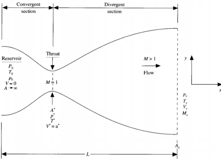
1. Converging-Diverging Nozzle Geometry:
- The nozzle features a carefully designed shape that includes a converging section, a throat, and a diverging section.
- The converging section accelerates the flow, leading to supersonic velocities at the throat.
- The diverging section allows for expansion, optimizing the flow for efficient supersonic propulsion.
2. Compressible Flow:
- The simulation considers the compressibility of the gas, which becomes significant at high velocities.
- Shock waves, expansion waves, and other compressible flow phenomena are expected and need to be accurately captured.
3. Shock Waves and Throat Conditions:
- Supersonic flows often involve shock waves, discontinuities that occur when the flow transitions from subsonic to supersonic or vice versa.
- The throat, where the cross-sectional area is smallest, is a critical point where the flow reaches its maximum velocity and conditions are most challenging.
4. Numerical Methods:
- Computational fluid dynamics (CFD) techniques, such as finite volume or finite difference methods, are commonly employed for 1D supersonic nozzle flow simulations.
- Time-marching algorithms and predictor-corrector methods are often used to solve the governing equations over discrete time steps.
5. Applications:
- Understanding supersonic nozzle flow is vital in the design and optimization of propulsion systems, including rocket engines and jet nozzles.
- These simulations contribute to the development of efficient and high-performance aerospace vehicles.
Matlab code :
Non Conservative function code :
Conservative function code :
Results :
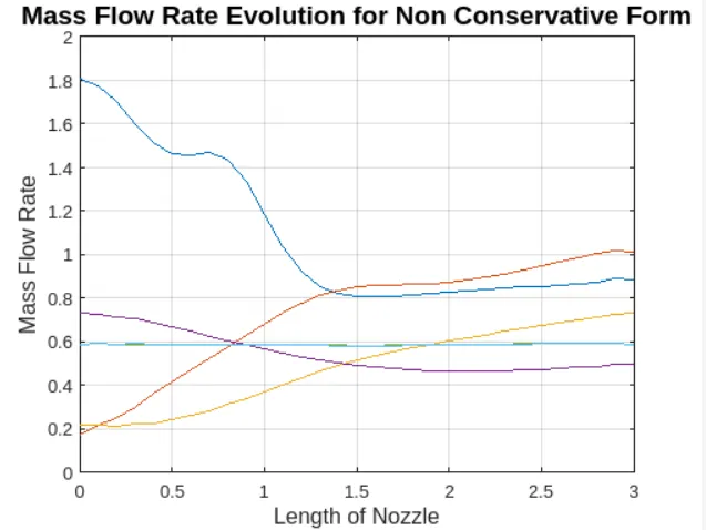
Figure 1 (Mass Flow Rate Evolution for Non-Conservative Form):
- Mass fow rates are plotted against the length of the nozzle for various time steps during the time marching process using the non-conservative form.
- The x-axis replresents the length of the nozzle, and the y-axis represents the mass flow rate.
- The plot is updated at different time steps (e.g., at time steps 50, 100, 150, 200, 700, and 1400).
Observations:
- Check how the mass flow rate evolves over time, particularly focusing on the nozzle's throat region.
- Observe whether the mass flow rate reaches a steady state or if there are any transient behaviors.
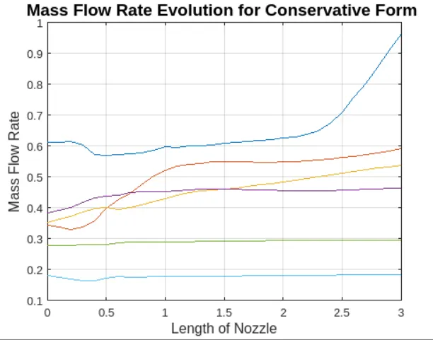
Figure 2 (Mass Flow Rate Evolution for Conservative Form):
- Similar to Figure 1, this figure represents the evolution of mass flow rates for various time steps but using the conservative form.
- The x-axis represents the length of the nozzle, and the y-axis represents the mass flow rate.
- The plot is updated at different time steps during the time marching process.
Observations:
- Compare the mass flow rate evolution between the non-conservative and conservative forms.
- Analyze whether the conservative form yields different results or converges differently compared to the non-conservative form.
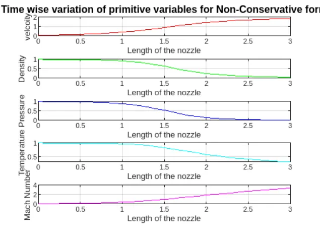
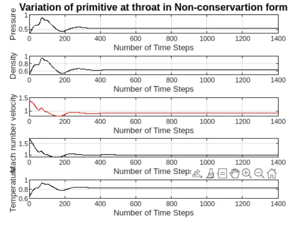
Non-Conservative Form Results (Figure 3 and Figure 4):
- Primitive Variables: Velocity, Density, Pressure, Temperature, and Mach Number are plotted against the length of the nozzle and for various time steps.
- The plots show the evolution of these variables over time using the non-conservative form of the governing equations.
- Throat Conditions: The primitive variables at the throat are also visualized for different time steps.
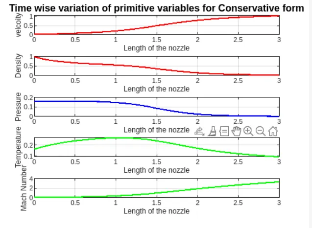
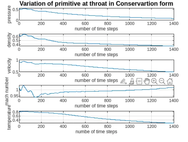
Conservative Form Results (Figure 5 and Figure 6):
- Similar to the non-conservative form, primitive variables are plotted against the length of the nozzle and for various time steps.
- Throat Conditions: The primitive variables at the throat are visualized over time using the conservative form.
Mass Flow Rate Variation (Figure 7):
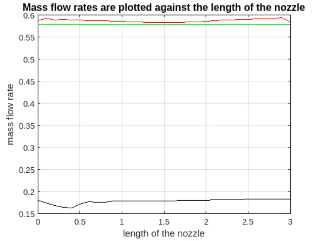
- Mass flow rates are plotted against the length of the nozzle for both non-conservative and conservative forms.
- The analytical solution is also included for reference.
- Observations: Check whether the mass flow rates converge to a steady-state value and how well the numerical results match the analytical solution.