Week 7 - Simulation of a 1D Supersonic nozzle flow simulation using Macormack Method

 Simulation of a 1D Supersonic nozzle flow simulation using the Macormack Method

Aim:

Simulate the isentropic flow through a quasi-1D subsonic-supersonic nozzle.

Derive the governing equations' conservation and non-conservation forms and solve them using MacCormack's technique.

Determine the steady-state temperature distribution for the flow-field variables and investigate the difference between the two forms of governing equations by comparing their solutions.

It would be best if you showed the following plots in the report
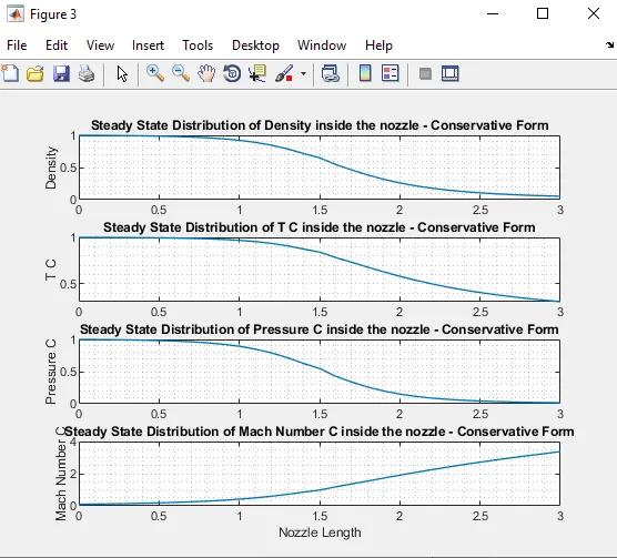
1. Steady-state distribution of primitive variables inside the nozzle
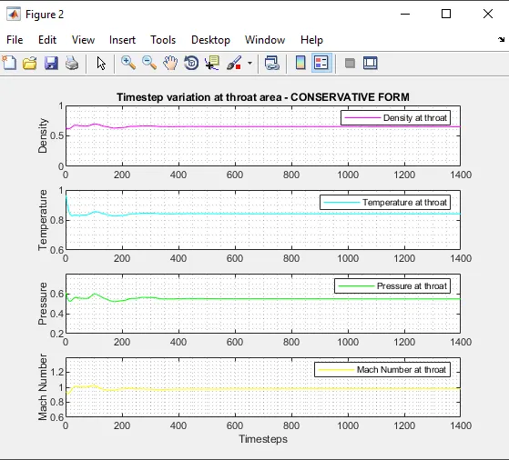
2. Time-wise variation of the primitive variables
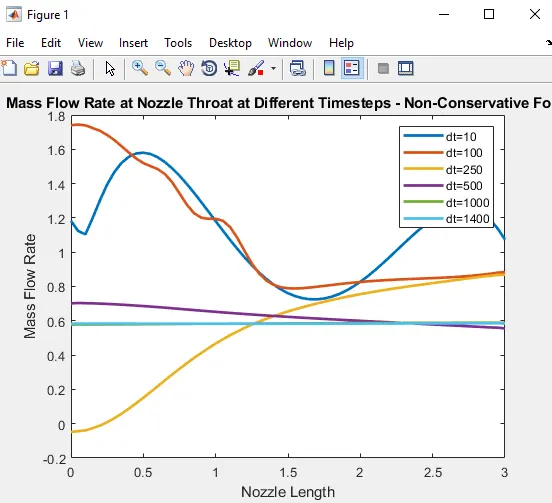
3. Variation of Mass flow rate distribution inside the nozzle at different time steps during the time-marching process
4. Comparison of Normalized mass flow rate distributions of both forms

Expected Results:

• Perform a grid independence test on the solution and explain all your findings.
• The code must be modular. It would help if you wrote separate functions to solve both forms.
• Discuss all the plots you are providing with observed inferences.  

Introduction

Nozzle

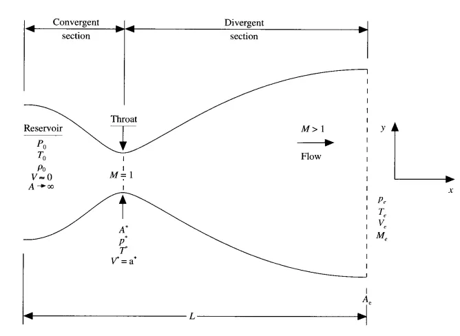
A nozzle is a device used to accelerate fluid flow, typically a gas or a liquid, by converting pressure energy into kinetic energy. Nozzles are commonly used in various engineering applications, such as rocket engines, jet engines, and steam turbines. They play a crucial role in directing and controlling the flow of fluids to achieve desired outcomes.

There are several types of nozzles

1. Converging Nozzle: This type of nozzle has a continuously decreasing cross-sectional area along its length. It accelerates the fluid by increasing its velocity while decreasing its pressure. Converging nozzles are often used in situations where the fluid is already at a high pressure.

2. Diverging Nozzle: A diverging nozzle has a continuously increasing cross-sectional area along its length. It decelerates the fluid, converting its kinetic energy back into pressure energy. Diverging nozzles are used in applications where the fluid is expanding, such as steam turbine exhausts.

3. Converging-Diverging (CD) Nozzle: Also known as a "de Laval" nozzle, the CD nozzle combines both converging and diverging sections. It is commonly used in rocket engines and supersonic jet engines. In the converging section, the fluid accelerates and its pressure decreases. As it enters the diverging section, the fluid expands and its velocity further increases, often reaching supersonic speeds.

4. Subsonic Nozzle: A subsonic nozzle operates at speeds lower than the local speed of sound. It is used in applications where the fluid remains below the speed of sound.

5. Subsonic Diffuser: While not strictly a nozzle, a subsonic diffuser is a device that gradually increases the cross-sectional area of a flow passage, causing the fluid to decelerate and its pressure to increase. It is often used to slow down and increase the pressure of a fluid.

Supersonic Nozzle: A supersonic nozzle is designed to accelerate the fluid to speeds higher than the local speed of sound. This type of nozzle is used in supersonic and hypersonic applications.

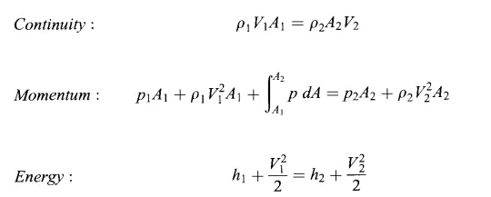
The governing continuity, momentum, and energy equation for the quasi-1D, steady, and isentropic flow can be expressed as

Conservative and Non-Conservative Form

Conservative and non-conservative forms are two different ways to represent certain mathematical equations, particularly those involving the conservation of physical quantities. These forms are commonly encountered in fluid dynamics, heat transfer, and other areas of physics and engineering.

Conservative Form:

The conservation of a certain quantity is specifically taken into account in the conservative form of an equation. Equations involving the conservation of mass, momentum, energy, and other conserved quantities frequently take this form. This variant of the equation states that the difference between the inflow and outflow rates plus the rate at which the quantity is generated or lost within the control volume equals how the quantity changes within a control volume. The conservative form makes sure that the conserved quantity's overall quantity within the control volume stays constant.

For example, the conservative form of the mass conservation equation (also known as the continuity equation) in fluid dynamics is:

∂ρ/∂t + ∇·(ρu) = 0

where ρ is the density of the fluid, u is the velocity vector, ∂ρ/∂t represents the rate of change of density with time, and ∇·(ρu) represents the divergence of the mass flow rate.

Non-Conservative Form:

The conservation of a particular quantity inside a control volume is implicit in the non-conservative version of an equation. Instead, it uses the local behavior of the relevant parameters to express the physical process. Even if the non-conservative form may be more logical and analytically straightforward, it does not ensure the overall conservation of the quantity under consideration, especially when complex systems with numerous interactions are taken into account.

In fluid dynamics, the non-conservative form of the mass conservation equation is expressed as:

∂ρ/∂t + ρ∇·u + u·∇ρ = 0

In this form, the second term (ρ∇·u) represents the local change in mass due to fluid flow, and the third term (u·∇ρ) accounts for the change in mass due to variations in density in the fluid flow.

Macormack Method:

A numerical method called the MacCormack method is used to solve time-dependent partial differential equations, especially those involving fluid dynamics and other physical processes. It is a predictor-corrector scheme that adds a corrective step to increase the explicit finite difference method's accuracy.

In order to solve hyperbolic conservation laws—which govern the conservation of mass, momentum, and energy in fluid flow as well as other wave-like phenomena—the approach is frequently used. When dealing with shock waves and other discontinuities, the MacCormack approach is particularly helpful.

1. Predictor Step:

   • Estimate the values of the dependent variables at the next time step using an explicit finite difference scheme.
   • This step involves estimating the "predicted" values of the dependent variables based on the current values and their spatial derivatives.

2. Corrector Step:

   • Estimate the values of the dependent variables at the intermediate time step.
   • Use the predicted values from the predictor step to estimate the intermediate values.

3. Final Step:

   • Recalculate the predicted values at the intermediate time step using the corrected values.
   • Update the dependent variables based on the corrected intermediate values.

The governing continuty, momentum and energy equations in terms of non dimensional variables for this quassi one dimensional staedy and isentropc flow can be expressed respectively as:

Non-Conservative Form:

Continuity equation

Momentum Equation

Energy Equation

Conservative Form:

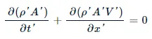
Momentum Equation

Energy Equation

Matlab Code 

Non-Conservative form

Function code

function [x, v, T, rho, M, P, mdot, M_thrt, rho_thrt, T_thrt, P_thrt, mdot_thrt, iteration_no, residual1, residual2, residual3] = NCF(n, x, gamma)
    dx = x(2) - x(1);
    
    rho_i = 1 - 0.3146 * x;
    T_i = 1 - 0.2314 * x;
    v_i = (0.1 + 1.09 * x) .* T_i.^0.5;
    A = 1 + 2.2 * (x - 1.5).^2;
    nzzl_thrt = find(A == 1);
    
    rho = rho_i;
    T = T_i;
    v = v_i;
    
    C = 0.5;
    dt = min(C * dx ./ (sqrt(T_i) + v_i));
    nt = 1400;
    
    for j = 1:nt
        rho_old = rho;
        v_old = v;
        T_old = T;
        
        for k = 2:n-1
            drho_dx = (rho(k+1) - rho(k)) / dx;
            dlnA_dx = (log(A(k+1)) - log(A(k))) / dx;
            dv_dx = (v(k+1) - v(k)) / dx;
            dT_dx = (T(k+1) - T(k)) / dx;
            
            drho_dt_p(k) = -(rho(k) * dv_dx) - (rho(k) * v(k) * dlnA_dx) - (v(k) * drho_dx);
            dv_dt_p(k) = -(v(k) * dv_dx) - (1/gamma) * (dT_dx + (T(k) / rho(k)) * drho_dx);
            dT_dt_p(k) = -(v(k) * dT_dx) - (gamma - 1) * T(k) * (dv_dx + v(k) * dlnA_dx);
            
            rho(k) = rho_old(k) + drho_dt_p(k) * dt;
            v(k) = v_old(k) + dv_dt_p(k) * dt;
            T(k) = T_old(k) + dT_dt_p(k) * dt;
        end
        
        for l = 2:n-1
            drho_dx = (rho(l) - rho(l-1)) / dx;
            dlnA_dx = (log(A(l)) - log(A(l-1))) / dx;
            dv_dx = (v(l) - v(l-1)) / dx;
            dT_dx = (T(l) - T(l-1)) / dx;
            
            drho_dt_c(l) = -(rho(l) * dv_dx) - (rho(l) * v(l) * dlnA_dx) - (v(l) * drho_dx);
            dv_dt_c(l) = -(v(l) * dv_dx) - (1/gamma) * (dT_dx + (T(l) / rho(l)) * drho_dx);
            dT_dt_c(l) = -(v(l) * dT_dx) - (gamma - 1) * T(l) * (dv_dx + v(l) * dlnA_dx);
        end
        
        for m = 2:n-1
            drho_dt(m) = 0.5 * dt * (drho_dt_p(m) + drho_dt_c(m));
            dv_dt(m) = 0.5 * dt * (dv_dt_p(m) + dv_dt_c(m));
            dT_dt(m) = 0.5 * dt * (dT_dt_p(m) + dT_dt_c(m));
            
            rho(m) = rho_old(m) + drho_dt(m);
            v(m) = v_old(m) + dv_dt(m);
            T(m) = T_old(m) + dT_dt(m);
        end
        
        v(1) = 2 * v(2) - v(3);
        rho(n) = 2 * rho(n-1) - rho(n-2);
        v(n) = 2 * v(n-1) - v(n-2);
        T(n) = 2 * T(n-1) - T(n-2);
        
        mdot = rho .* v .* A;
        M = v ./ sqrt(T);
        P = rho .* T;
        
        rho_thrt(j) = rho(nzzl_thrt);
        T_thrt(j) = T(nzzl_thrt);
        P_thrt(j) = P(nzzl_thrt);
        M_thrt(j) = M(nzzl_thrt);
        mdot_thrt(j) = rho(nzzl_thrt) * v(nzzl_thrt) * A(nzzl_thrt);
        iteration_no(j) = j;
        
        residual1(j) = drho_dt(nzzl_thrt);
        residual2(j) = dv_dt(nzzl_thrt);
        residual3(j) = dT_dt(nzzl_thrt);
        
        if j == 10 || j == 100 || j == 250 || j == 500 || j == 1000 || j == 1400
            plot(x, mdot, 'LineWidth', 2);
            hold on;
        end
    end
    
    xlabel('Nozzle Length');
    ylabel('Mass Flow Rate');
    legend('dt=10', 'dt=100', 'dt=250', 'dt=500', 'dt=1000', 'dt=1400');
    title('Mass Flow Rate at Nozzle Throat at Different Timesteps - Non-Conservative Form');
end


Main Code

% Quasi 1D Supersonic Nozzle Flow using MacCormack method

% Clear the workspace, close all figures, and clear the command window
clear all
close all
clc

�fine the number of nodes and generate an array representing the domain length
n = 61;
x = linspace(0, 3, n);

�fine the specific heat ratio
gamma = 1.4;

% Prompt the user to choose the simulation method (1 for Non-Conservative Form, 2 for Conservative Form)
method = input('Enter (1) for Non-Conservative Form and (2) for Conservative Form: ');

% Check the chosen method and perform respective calculations
if method == 1
    �ll the NCF function to compute the Non-Conservative Form results
    [x, v, T, rho, M, P, mdot, M_thrt, rho_thrt, T_thrt, P_thrt, mdot_thrt, iteration_no, residual1, residual2, residual3] = NCF(n, x, gamma);

    % Create Figure 2 and set up subplot labels and property data
    figure(2)
    subplot_labels = {'Mach Number', 'Pressure Ratio', 'Temperature Ratio', 'Density Ratio', 'Mass Flow Rate'};
    properties_data = {M, P, T, rho, mdot};

    % Loop through properties and create subplots
    for i = 1:5
        subplot(5, 1, i) % Set up subplot
        plot(x, properties_data{i}, 'LineWidth', 2) % Plot property data
        ylabel(subplot_labels{i}) % Set y-label
        if i == 5
            xlabel('Nozzle Length') % Set x-label for the last subplot
        end
        grid on % Display grid lines
        title(['Steady-State Distribution of ' subplot_labels{i} ' inside the nozzle - Non-Conservative Form']) % Set title
    end

    % Create Figure 3 and plot throat properties over time
    figure(3)
    plot(iteration_no, M_thrt, iteration_no, rho_thrt, iteration_no, T_thrt, iteration_no, P_thrt, iteration_no, mdot_thrt, 'LineWidth', 2)
    grid on
    xlabel('Number of Timesteps')
    legend('Mach Number', 'Density Ratio', 'Temperature Ratio', 'Pressure Ratio', 'Mass flow rate')
    title('Time-wise variation of variable at nozzle throat - Non-Conservative Form')

    % Create Figure 4 and plot residual values over time
    figure(4)
    plot(iteration_no, residual1, iteration_no, residual2, iteration_no, residual3, 'LineWidth', 2)
    grid on
    xlabel('Number of Timesteps')
    ylabel('Residuals')
    legend('Density Ratio Residuals', 'Velocity Ratio Residuals', 'Temperature Ratio Residuals')
    title('Residual Values - Non-Conservative Form')

% If method is not 1, display an error message
else
    disp('Invalid Input')
end

OUTPUT

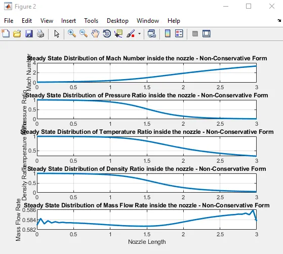
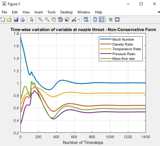
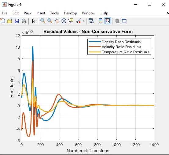
Conservative Form

Matlab Code

Function Code

function [Mass_flow_rate_C, Pressure_C, Mach_number_C,  rho_C, v_C, T_C, rho_throat_C, v_throat_C, T_throat_C, Mass_flow_rate_throat_C, Pressure_throat_C, Mach_number_throat_C] = Conservative_form1(x, dx, n, gamma, nt, C)

�termining Initial profile of Density and Temperature
for i = 1:n
    
    if (x(i) >= 0 && x(i) <= 0.5)
        rho_C(i) = 1;
        T_C(i) = 1;
    elseif (x(i) >= 0.5 && x(i) <= 1.5)
        rho_C(i) = 1 - 0.366*(x(i) - 0.5);
        T_C(i) = 1 - 0.167*(x(i) - 0.5);
    elseif (x(i) >= 1.5 && x(i) <= 3)
        rho_C(i) = 0.634 - 0.3879*(x(i) - 1.5);
        T_C(i) = 0.833 - 0.3507*(x(i) - 1.5);
    end
    
end

%Area & Throat profiles
a = 1 + 2.2*(x - 1.5).^2;
throat = find(a==1);

%Initial profile fot Velocity and Pressure
v_C = 0.59./(rho_C.*a);
Pressure_C = rho_C.*T_C;

�lculate the Initial Solution Vectors(U)
U1 = rho_C.*a;
U2 = rho_C.*a.*v_C;
U3 = rho_C.*a.*(T_C./(gamma - 1)) + ((gamma/2).*v_C.^2);

%Outer Time Loop
for k =1:nt
    
    %Time-step control
    dt = min(C.*dx./(sqrt(T_C) + v_C));
    
    %Saving a copy of Old Values
    U1_old = U1;
    U2_old = U2;
    U3_old = U3;

    �lculating the Flux vector(F)
    F1 = U2;
    F2 = ((U2.^2)./U1) + ((gamma - 1)/gamma)*(U3 - (gamma/2)*((U2.^2)./U1));
    F3 = ((gamma*U2.*U3)./U1) - (gamma*(gamma - 1)*((U2.^3)./(2*U1.^2)));
    
    
    %Predictor Method
    for j = 2:n-1
    
        �lculating the Source term(J)
        J2(j) = (1/gamma)*rho_C(j)*T_C(j)*((a(j + 1) - a(j))/dx);
        
        
        %Continuity Equation
        dU1_dt_P(j) = -((F1(j + 1) - F1(j))/dx);
        
        %Momentum Equation
        dU2_dt_P(j) = -((F2(j + 1) - F2(j))/dx) + J2(j);
        
        %Energy Equation
        dU3_dt_P(j) = -((F3(j + 1) - F3(j))/dx);
        
        
        %Updating New values
        U1(j) = U1(j) + dU1_dt_P(j)*dt;
        U2(j) = U2(j) + dU2_dt_P(j)*dt;
        U3(j) = U3(j) + dU3_dt_P(j)*dt;
        
    end
    
    %Updating Flux vectors
    F1 = U2;
    F2 = ((U2.^2)./U1) + ((gamma - 1)/gamma)*(U3 - ((gamma*0.5*(U2.^2))./(U1)));
    F3 = ((gamma*U2.*U3)./U1) - ((gamma*0.5*(gamma - 1)*(U2.^3))./(U1.^2));

    
    %Corrector Method
    for j = 2:n-1
        
        %Updating the Source term(J)
        J2(j) = (1/gamma)*rho_C(j)*T_C(j)*((a(j) - a(j - 1))/dx);

        %Simplifying the Equation's spatial terms
        dU1_dt_C(j) = -((F1(j) - F1(j - 1))/dx);
        dU2_dt_C(j) = -((F2(j) - F2(j - 1))/dx) + J2(j);
        dU3_dt_C(j) = -((F3(j) - F3(j - 1))/dx);

    end

    %Compute Average Time derivative
    dU1_dt = 0.5*(dU1_dt_P + dU1_dt_C);
    dU2_dt = 0.5*(dU2_dt_P + dU2_dt_C);
    dU3_dt = 0.5*(dU3_dt_P + dU3_dt_C);

    %Final Solution Update
    for i = 2:n-1
        U1(i) = U1_old(i) + dU1_dt(i)*dt;
        U2(i) = U2_old(i) + dU2_dt(i)*dt;
        U3(i) = U3_old(i) + dU3_dt(i)*dt;
        
    end
    
    
    %Applying Boundary Conditions
    %At Inlet
    U1(1) = rho_C(1)*a(1);
    U2(1) = 2*U2(2) - U2(3);
    
    v_C(1) = U2(1)./U1(1);
    U3(1) = U1(1)*((T_C(1)/(gamma - 1)) + ((gamma/2)*(v_C(1)).^2));
    
    %At Outlet
    U1(n) = 2*U1(n - 1) - U1(n - 2);
    U2(n) = 2*U2(n - 1) - U2(n - 2);
    U3(n) = 2*U3(n - 1) - U3(n - 2);
    
    %Final Primitive value update
    rho_C = U1./a;
    v_C = U2./U1;
    T_C = (gamma - 1)*((U3./U1 - (gamma/2)*(v_C).^2));
    
    �fining Mass flow rate, Pressure and Mach number
    Mass_flow_rate_C = rho_C.*a.*v_C;
    Pressure_C = rho_C.*T_C;
    Mach_number_C = (v_C./sqrt(T_C));
    
    �lculating Variables at throat section
    rho_throat_C(k) = rho_C(throat);
    T_throat_C(k) = T_C(throat);
    v_throat_C(k) = v_C(throat);
    Mass_flow_rate_throat_C(k) = Mass_flow_rate_C(throat);
    Pressure_throat_C(k) = Pressure_C(throat);
    Mach_number_throat_C(k) = Mach_number_C(throat);
    
    %PLOTTING
    %Comparison of non-dimensional Mass flow rates at different time steps
    figure(1)
    if k == 50
       plot(x, Mass_flow_rate_C, 'm', 'linewidth', 1.25);
       hold on
    elseif k == 100
       plot(x, Mass_flow_rate_C, 'c', 'linewidth', 1.25);
       hold on
    elseif k == 200
       plot(x, Mass_flow_rate_C, 'g', 'linewidth', 1.25);
       hold on
    elseif k == 400
       plot(x, Mass_flow_rate_C, 'y', 'linewidth', 1.25);
       hold on
    elseif k == 800
       plot(x, Mass_flow_rate_C, 'k', 'linewidth', 1.25);
       hold on
    end
    
    %Labelling
    title('Mass flow rates at different Timesteps - CONSERVATIVE FORM')
    xlabel('Distance')
    ylabel('Mass flow rate')
    legend({'50^t^h Timestep','100^t^h Timestep','200^t^h Timestep','400^t^h Timestep','800^t^h Timestep'})
    axis([0 3 0.4 1])
    grid on

end

end

Main Code

% Clear the workspace, close all figures, and clear the command window
clear all
close all
clc

�fine the number of nodes and generate an array representing the domain length
n = 31;
x = linspace(0, 3, n);
dx = x(2) - x(1);
nt = 1400;

% Courant Number
C = 0.5;

�fine the specific heat ratio
gamma = 1.4;

%FUNCTION FOR CONSERVATIVE FORM
tic;
[Mass_flow_rate_C, Pressure_C, Mach_number_C,  rho_C, v_C, T_C, rho_throat_C, v_throat_C, T_throat_C, Mass_flow_rate_throat_C, Pressure_throat_C, Mach_number_throat_C] = Conservative_form1(x, dx, n, gamma, nt, C)
Time_elasped_C = toc;
fprintf('Time Elasped for Conservative form: %0.4f', Time_elasped_C);

%PLOTTING 
%Timestep variation of properties at throat area in Conservative form
figure(2)

�nsity
subplot(4,1,1)
plot(rho_throat_C,'color','m')
ylabel('Density')
legend({'Density at throat'})
axis([0 1400 0 1])
grid minor
title('Timestep variation at throat area - CONSERVATIVE FORM')

%Temperature
subplot(4,1,2)
plot(T_throat_C,'color','c')
ylabel('Temperature')
legend({'Temperature at throat'})
axis([0 1400 0.6 1])
grid minor

%Pressure
subplot(4,1,3)
plot(Pressure_throat_C,'color','g')
ylabel('Pressure')
legend({'Pressure at throat'})
axis([0 1400 0.2 0.8])
grid minor

%Mach Number
subplot(4,1,4)
plot(Mach_number_throat_C,'color','y')
xlabel('Timesteps')
ylabel('Mach Number')
legend({'Mach Number at throat'})
axis([0 1400 0.6 1.4])
grid minor

% Create Figure and set up subplot labels and property data
    figure(3)
    subplot_labels = {'Density', 'T C', 'Pressure C', 'Mach Number C'};
    properties_data = {rho_C, T_C, Pressure_C, Mach_number_C};

    % Loop through properties and create subplots
    for i = 1:4
        subplot(4, 1, i) % Set up subplot
        plot(x, properties_data{i}, 'LineWidth', 1) % Plot property data
        ylabel(subplot_labels{i}) % Set y-label
        if i == 4
            xlabel('Nozzle Length') % Set x-label for the last subplot
        end
        grid minor % Display grid lines
        title(['Steady-State Distribution of ' subplot_labels{i} ' inside the nozzle - Conservative Form']) % Set title
    end

Output

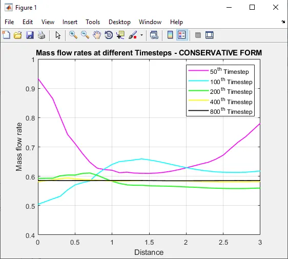
Conclusion

1. In our simulation, the decision between conservative and non-conservative forms reveals intriguing trade-offs.
2. The conservative technique is superior at maintaining the mass flow distribution whereas the non-conservative approach offers a little bit more precision in primitive variables. This illustrates its natural capacity to efficiently conserve mass.
3. Notably, the non-conservative method produces fewer residuals, which are often a sign of a good solution. In contrast to the conservative approach, which calls for additional steps to decode primitive variables from flow variables, it requires less computational work.
4. While the non-conservative technique can catch up with larger timesteps, the conservative form ultimately proves to be the most accurate and trustworthy choice.