Week 7 - Simulation of a 1D Supersonic nozzle flow simulation using Macormack Method
AIM:
To simulate the isentropic flow through a quasi 1D subsonic-supersonic nozzle and derive both the conservation and non-conservation forms of the governing equations and sovle them using the MacCormack's technique
objectives:
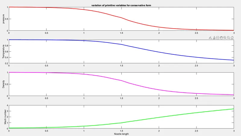
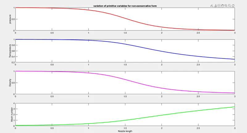
1. Steady-state distribution of primitive variables inside the nozzle
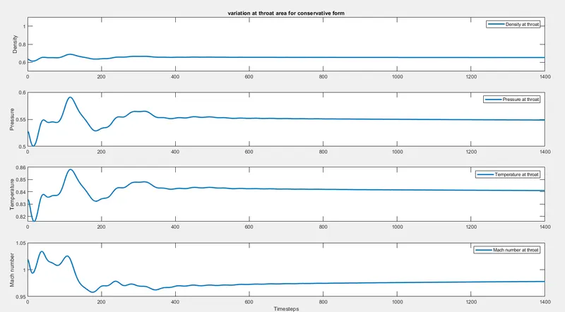
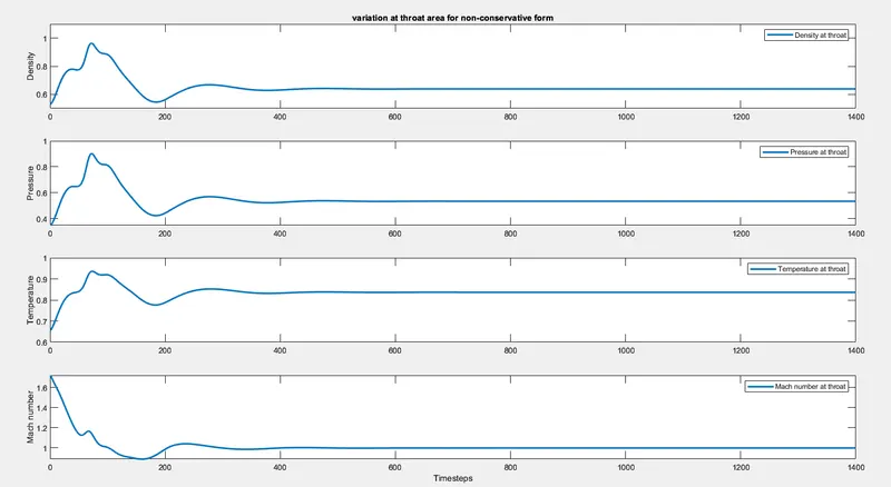
2. Time-wise variation of the primitive variables
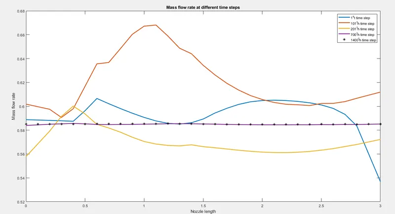
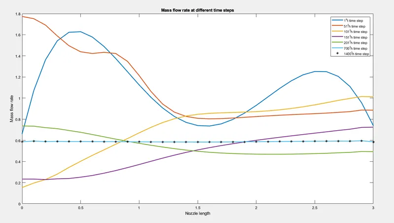
3. Variation of Mass flow rate distribution inside the nozzle at different time steps during the time-marching process
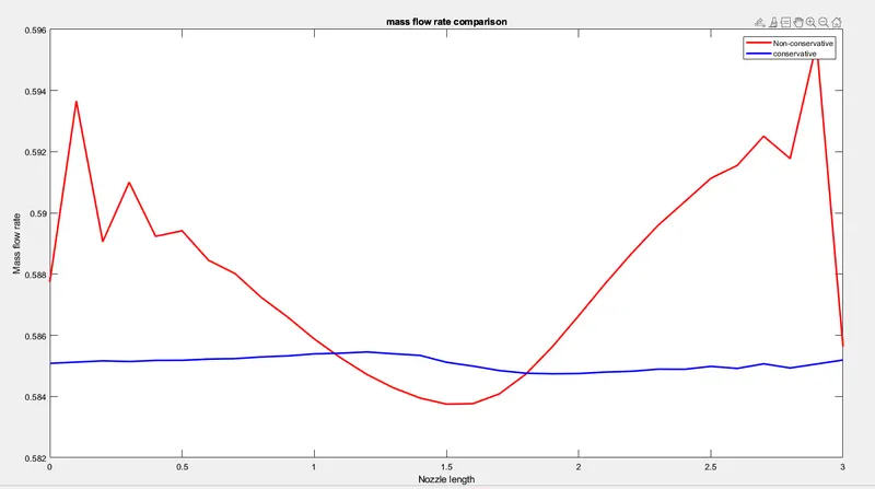
4. Comparison of Normalized mass flow rate distributions of both forms
Theory:
Consider an isentropic flow through a convergent-divergent nozzle. Flow at the inlet to the nozzle comes from the reservior.
The cross sectional area of the reservior is large which means A tends to infinity and velocity is very small which tends to zero.
The flow expands isentropically to the supersonic speeds at the nozzle exit and the flow is locally subsonic in the convergent section section of the nozzle, sonic at the throat and supersonic at the divergent section.
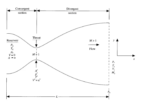
We assume that at a given section, the cross sectional area A, the flow properties are uniform across that section.
Area of the nozzle changes as a function of distance along the nozzle x.
We assume that the flow properties are vary only with x. and assuming the uniform flow properties across any given cross section so thats why its called quasi one dimensional flow.
Governing equations are represented in terms of PDE for both forms, here we have to do time marching in this problem so that the governing equations are interms of non-dimensional varianles which is expressed below.
Non-conservative form:
continuity equation
`(delrho')/(delt') =-rho'((delV')/(delx'))-rho'V'((del(lnA))/(delx'))-V'((delrho')/(delx'))`
Momentum equation
`(delV')/(delt')=-V'((delV')/(delx'))-(1/gamma)((delT')/(delx')+(T')/(rho')((delrho')/(delx')))`
Energy equation
`(delT')/(delt')=-V'(delT')/(delx')-(gamma-1)T'[(delV')/(delx')+V'(del(lnA'))/(delx')]`
Conservative form
`(del(rho'A'))/(delt')+(del(rho'A'V'))/(delx')=0`
Momentum equation
`(del(rho'A'V'))/(delt')+(del[rho'A'(V')^2+(1/gamma)rho'A'])/(delx')=(1/gamma)rho'((delA')/(delx'))`
Energy equation

Maccormack method:
In this method, we split Time marching into predictor and corrector phases.
Initial conditions:
The initial profile for all the flow variables which are velocity, density and temperature has to be determined
Predictor step
`((delf)/(delt))=f(i+1-f(i))/(Deltax)`
Solution update
`f_p=f_i+(delf)/(delt).Deltat`
f_p=flow field variables claculated after the predictor step
f_i=flow field variables in the initial step.
`Deltat`=time step size.
Corrector step
`(delf)/(dt)=(f(i)-f(i-1))/(Deltax)`
Average time derivative
`(delf)/(dt)=0.5(((delf)/(dt))_p+((delf)/(dt))_c)`
Final solution update
f_sol=f_initial+(delf/delt)avg.Delt
Main program:
clear all
close all
clc

L=3;
n=31;
nt=1:1400;
cfl=0.5;
x=linspace(0,L,n);

%calling function program of non-conservative form
[mass_flow_rate_nc,mass_flow_rate_throat_nc]=non_conservative(L,n,nt,cfl)

%calling function program of conservative form
[mass_flow_rate_c,mass_flow_rate_throat_c]=conservative(L,n,nt,cfl)


%plot for mass flow rate comparison
figure(7)
plot(x,mass_flow_rate_nc,'r','LineWidth',2)
hold on
plot(x,mass_flow_rate_c,'b','LineWidth',2)
legend('Non-conservative','conservative')
title('mass flow rate comparison')
xlabel('Nozzle length')
ylabel('Mass flow rate')
Here we defining the length of the nozzle, number of node points , mesh size with these we creating the domain
And here we calling the function program of conservative and non-conservative form.
And we have a comparision plot for conservative and non-conservative form.
Non_conservative function program:
function [mass_flow_rate_nc,mass_flow_rate_throat_nc]=non_conservative(L,n,nt,cfl)


x=linspace(0,L,n);
dx=x(2)-x(1);

%initial conditions
rho=1-0.3146*x;
T=1-0.2314*x;
V=(0.1+1.09*x).*T.^0.5;
A=1+2.2*(x-1.5).^2;

M=V./(T.^0.5);
mass_flow_rate=rho.*A.*V;
p=rho.*T;
gamma=1.4;

%Time step
for z=1:31
    a=(T(z))^0.5;
    dt(z)=cfl*dx/(a+V(z));
end
dt=min(dt);

%Time loop
for i=1:length(nt)

    rho_old=rho;
    T_old=T;
    V_old=V;

%space loop
    % predictor step
 for j=2:n-1
        dvdx=(V(j+1)-V(j))/dx;
        drhodx=(rho(j+1)-rho(j))/dx;
        dtdx=(T(j+1)-T(j))/dx;
        dlogadx=(log(A(j+1))-log(A(j)))/dx;
        %continuity
        drhodt_p(j)=-rho(j)*dvdx-rho(j)*V(j)*dlogadx-V(j)*drhodx;
        %momentum
        dvdt_p(j)=-V(j)*dvdx-(1/gamma)*(dtdx+(T(j)/rho(j))*drhodx);
        %Energy
        dTdt_p(j)=-V(j)*(dtdx)-(gamma-1)*T(j)*(dvdx+V(j)*dlogadx);


        %solution update
        %continuity
        rho(j)=rho(j)+drhodt_p(j)*dt;
        %momentum
        V(j)=V(j)+dvdt_p(j)*dt;
        %energy
        T(j)=T(j)+dTdt_p(j)*dt;


  % corrector step
        dvdx=(V(j)-V(j-1))/dx;
        drhodx=(rho(j)-rho(j-1))/dx;
        dtdx=(T(j)-T(j-1))/dx;
        dlogadx=(log(A(j))-log(A(j-1)))/dx;
        %continuity
        drhodt_c(j)=-rho(j)*dvdx-rho(j)*V(j)*dlogadx-V(j)*drhodx;
        %momentum
        dvdt_c(j)=-V(j)*dvdx-(1/gamma)*(dtdx+(T(j)/rho(j))*drhodx);
        %Energy
        dTdt_c(j)=-V(j)*(dtdx)-(gamma-1)*T(j)*(dvdx+V(j)*dlogadx);
   end

    % average time derivative
drhodt=0.5*(drhodt_p+drhodt_c);
dvdt=0.5*(dvdt_p+dvdt_c);
dTdt=0.5*(dTdt_p+dTdt_c);

 % final solution update
for k=2:n-1

    rho(k)=rho_old(k)+drhodt(k)*dt;
    V(k)=V_old(k)+dvdt(k)*dt;
    T(k)=T_old(k)+dTdt(k)*dt;
end

%apply boundary condition
%inlet
V(1)=2*V(2)-V(3);

%outlet
rho(n)=2*rho(n-1)-rho(n-2);
V(n)=2*V(n-1)-V(n-2);
T(n)=2*T(n-1)-T(n-2);

%Final update of old values
p=rho.*T;
M=V./T.^0.5;
mass_flow_rate=rho.*A.*V

%Finding values at throat point
T_throat(i)=T(16);
rho_throat(i)=rho(16);
V_throat(i)=V(16);
M_throat(i)=M(16);
p_throat(i)=p(16);
mass_flow_rate_throat(i)=mass_flow_rate(16);


%Plotting
%comparision of non-dimensional mass flow rates at different time steps

for w=[1:50:201 700]
    if w==i
      figure(1)
       plot(x,mass_flow_rate,'lineWidth',2)
       xlabel('Nozzle length')
       ylabel('Mass flow rate')
       title('Mass flow rate at different time steps')
       hold on

   elseif i==1400
        plot(x,mass_flow_rate,'*black')
        legend('1^st time step','51^th time step','101^th time step','151^th time step','201^th time step','700^th time step','1400^th time step')
    end
end

end


figure(2)
%pressure
subplot(4,1,1)
plot(x,p,'r','LineWidth',2)
ylabel('pressure')
title('variation of primitive variables for non-conservative form')


%Temperature
subplot(4,1,2)
plot(x,T,'b','LineWidth',2)
ylabel('Temperature')


%Density
subplot(4,1,3)
plot(x,rho,'m','LineWidth',2)
ylabel('Density')


%Mach number
subplot(4,1,4)
plot(x,M,'g','LineWidth',2)
xlabel('Nozzle length')
ylabel('Mach number')


figure(3)
%Timestep variation of rho,T,p and Mach number at the nozzle throat
%Density at throat
subplot(4,1,1)
plot(nt,rho_throat,'LineWidth',2)
ylabel('Density')
legend('Density at throat')
axis([0 1400 0.5 1.1])
title('variation at throat area for non-conservative form')
hold on

%Pressure at throat
subplot(4,1,2)
plot(nt,p_throat,'linewidth',2)
ylabel('Pressure')
legend('Pressure at throat')

%Temperature at throat
subplot(4,1,3)
plot(nt,T_throat,'linewidth',2)
ylabel('Temperature')
legend('Temperature at throat')

%Mach number at throat
subplot(4,1,4)
plot(nt,M_throat,'linewidth',2)
xlabel('Timesteps')
ylabel('Mach number')
legend('Mach number at throat')


mass_flow_rate_nc=mass_flow_rate;
mass_flow_rate_throat_nc=mass_flow_rate_throat;
end
Coding explanation
In this Non_conservative function program we used to calculate the values of mass flow rate and mass flow rate of throat area for all grid points.
We have an initial conditions for density, Temperature, velocty and area of the profile. so with these initial conditions we start the time marching.
Calculating the Mach number (M=V./(T.^0.5) which is dimensionless number defined as the local velocity to the localspeed of sound. based on the initial conditions we calculate mass flow flow rate and pressure(p=rho.*T)
Calculating the time step inside the for loop for all grid points.
function [mass_flow_rate_c,mass_flow_rate_throat_c]=conservative(L,n,nt,cfl)


x=linspace(0,L,n);
dx=x(2)-x(1);

%initial conditions
for q=1:length(x)

    if (x(q)<=0.5)
        rho(q)=1;
        T(q)=1;
    elseif (x(q)>0.5) & (x(q)<=1.5)
        rho(q)=1-0.366*(x(q)-0.5);
        T(q)=1-0.167*(x(q)-0.5);
    elseif (x(q)>1.5) & (x(q)<=3.5);
        rho(q)=0.634-0.3879*(x(q)-1.5);
        T(q)=0.833-0.3507*(x(q)-1.5);
    end
end

A=1+2.2*(x-1.5).^2;    %nozzle profile
gamma=1.4;

%solution vector u1,u2,u3
u1=rho.*A;
u2=0.59*ones(1,n);
V=u2./u1;
u3=u1.*((T./(gamma-1))+(gamma/2).*V.^2);


M=V./(T.^0.5);
mass_flow_rate=rho.*A.*V;
p=rho.*T;

%loop for time step
for z=1:31
    a=(T(z))^0.5;
    dt(z)=cfl*dx/(a+V(z));
end
dt=min(dt);

%Time loop
for i=1:length(nt)

    u1_old=u1;
    u2_old=u2;
    u3_old=u3;

    for j=2:n-1
        %flux vector calculation
        f1=u2;
        f2=((u2.^2)./u1)+((gamma-1)/gamma)*(u3-((gamma/2)*(u2.^2)./u1));
        f3=((gamma.*u2.*u3)./u1)-((gamma*(gamma-1)/2)*(u2.^3)./(u1.^2));

        %source term calculation
        j1=(1/gamma)*rho(j)*T(j)*((A(j+1)-A(j))/dx);

        %predictor step
        %contimuity equation
        du1_dt_p(j)=-(f1(j+1)-f1(j))/dx;

        %momentum equation
        du2_dt_p(j)=-(f2(j+1)-f2(j))/dx+j1;

        %energy equation
        du3_dt_p(j)=-(f3(j+1)-f3(j))/dx;

        %updating solution vectors
        u1(j)=u1_old(j)+du1_dt_p(j)*dt;
        u2(j)=u2_old(j)+du2_dt_p(j)*dt;
        u3(j)=u3_old(j)+du3_dt_p(j)*dt;

        %updating primitive values
        rho=u1./A;
        %V=u2./u1;
        T=(gamma-1).*(u3./u1-(gamma/2).*(u2./u1).^2);

        %updating flux terms
        f1=u2;
        f2=u2.^2./u1+((gamma-1)/gamma)*(u3-(gamma/2)*u2.^2./u1);
        f3=((gamma.*u2.*u3)./u1)-((gamma*(gamma-1)/2)*(u2.^3)./(u1.^2));
       % f3=gamma.*u2.*u3./u1-0.5*gamma*(gamma-1).*u2.^3./u1.^2;


        %corrector step
          j2=(1/gamma)*(rho(j)*T(j)*(A(j)-A(j-1))/dx);

          du1_dt_c(j)=-(f1(j)-f1(j-1))/dx;
          du2_dt_c(j)=-(f2(j)-f2(j-1))/dx+j2;
          du3_dt_c(j)=-(f3(j)-f3(j-1))/dx;

    end

    %average time derivative
            du1_dt=0.5*(du1_dt_p+du1_dt_c);
            du2_dt=0.5*(du2_dt_p+du2_dt_c);
            du3_dt=0.5*(du3_dt_p+du3_dt_c);

            %final corrected values

            for k=2:n-1
                u1(k)=u1_old(k)+du1_dt(k)*dt;
                u2(k)=u2_old(k)+du2_dt(k)*dt;
                u3(k)=u3_old(k)+du3_dt(k)*dt;

            end

            %inflow boundary conditions
            u1(1)=A(1);
            u2(1)=2*u2(2)-u2(3);
            u3(1)=u1(1)*(T(1)/(gamma-1)+(gamma*(u2(1)/u1(1))^2)/2);

            %outflow boundary conditions
            u1(n)=2*u1(n-1)-u1(n-2);
            u2(n)=2*u2(n-1)-u2(n-2);
            u3(n)=2*u3(n-1)-u3(n-2);

            %Final primitive update
        rho=u1./A;
        V=u2./u1;
        T=(gamma-1).*(u3./u1-(gamma/2).*(u2./u1).^2);
        p=rho.*T;
        M=V./T.^0.5;
        mass_flow_rate=u2;

%find values at throat point
T_throat(i)=T(16);
rho_throat(i)=rho(16);
V_throat(i)=V(16);
M_throat(i)=M(16)
p_throat(i)=p(16);
mass_flow_rate_throat(i)=mass_flow_rate(16);


%Plotting
%comparision of non-dimensional mass flow rates at different time steps
for w=[1:100:201 700]
    if w==i
      figure(4)
       plot(x,mass_flow_rate,'lineWidth',2)
       xlabel('Nozzle length')
       ylabel('Mass flow rate')
       title('Mass flow rate at different time steps')
       hold on

    elseif i==1400
        plot(x,mass_flow_rate,'*black')
        legend('1^st time step','101^th time step','201^th time step','700^th time step','1400^th time step')
    end
end


end

figure(5)

%pressure
subplot(4,1,1)
plot(x,p,'r','LineWidth',2)
ylabel('pressure')
title('variation of primitive variables for conservative form')

%Temperature
subplot(4,1,2)
plot(x,T,'b','LineWidth',2)
ylabel('Temperature')


%Density
subplot(4,1,3)
plot(x,rho,'m','LineWidth',2)
ylabel('Density')


%Mach number
subplot(4,1,4)
plot(x,M,'g','LineWidth',2)
xlabel('Nozzle length')
ylabel('Mach number')


figure(6)
%Timestep variation of rho,T,p and Mach number at the nozzle throat
%Density at throat
subplot(4,1,1)
plot(nt,rho_throat,'LineWidth',2)
ylabel('Density')
legend('Density at throat')
axis([0 1400 0.5 1.1])
title('variation at throat area for conservative form')
hold on

%Pressure at throat
subplot(4,1,2)
plot(nt,p_throat,'linewidth',2)
ylabel('Pressure')
legend('Pressure at throat')

%Temperature at throat
subplot(4,1,3)
plot(nt,T_throat,'linewidth',2)
ylabel('Temperature')
legend('Temperature at throat')

%Mach number at throat
subplot(4,1,4)
plot(nt,M_throat,'linewidth',2)
xlabel('Timesteps')
ylabel('Mach number')
legend('Mach number at throat')

mass_flow_rate_c=mass_flow_rate;
mass_flow_rate_throat_c=mass_flow_rate_throat;
end
Coding explanation
- Here the initial conditions for density and temperature are determined inside the for loop using if and ifelse statement.
- Governing equations are split into solution vector(u), Flux vector(F) and source terms(j) in order to simplify it.
- Calculating the time step inside the for loop for all grid points.
- dt(z)=cfl*dx/(a+V(z)) where cfl is the courant number which is considered as necessary condition for convergence while solving certain partial differential equations usually hyperbolic pdes numerically using explicit time marching schemes. a- local speed of sound and v is velocity.
- In outer time loop we computing the profile at different time steps.
- Maccormack technique is applied to solve the continuity, Momentum and energy equations of conservative form.
- Before that we calculate the flux vector and source terms inside the space loop.
- After the predictor step we updating the solution vector, updating primitive variables and flux terms inside the same space loop.
- After the end of predictor and corrector steps, calculated values are averaged in the next step and updating the final solution update.
- Apply the boundary conditions for calculating the mass flow rate, pressure, mach number and also calculating the values at throat area.
- Plotting the mass flow rate at different time steps and primitive variables are plotted for nozzle length and also plotted throat area variation in primitives variables against time steps.