Week 4.1 - Genetic Algorithm

GENETIC ALGORITHM

Aim:

TO write a program to calculate the global maxima of a stalagmite function using genetic algorithm.

Objective:

By using equation of stalagmite function and genetic algorithm syntax to calculate the global maxima.

Genetic Algorithm:

Genetic Algorithm is a search-based optimization technique, inspired by Charles Darwin’s theory of natural evolution. This algorithm reflects the process of natural selection where the fittest individuals are selected for reproduction in order to produce offspring of the next generation.

Optimization helps to find the better output from the set of ‘n’ number of inputs.

Operators of Genetic Algorithms

Once the initial generation is created, the algorithm evolves the generation using following operators –
1) Selection Operator: The idea is to give preference to the individuals with good fitness scores and allow them to pass their genes to the successive generations.
2) Crossover Operator: This represents mating between individuals. Two individuals are selected using selection operator and crossover sites are chosen randomly. Then the genes at these crossover sites are exchanged thus creating a completely new individual (offspring)`

3)Mutation

After the crossover, for each of the genes of the chromosomes (except for the elite chromosome), the gene will be mutated to any one of the codes with a probability of MutationProb. With the crossover and mutations completed, the chromosomes are once again evaluated for another round of selection and reproduction.

Genetic algorithm syntax

• X=ga(fun,nvars)

Fun-function name

vars- number of variables

Genetic algorithm always gives local minima value

• X=ga(fun,nvars,A,B,Aeq,lb,ub)

The above syntax defines a set of lower and upper bounds on the designed variables x.

• X=ga(fun,nvars,A,B,Aeq,Beq,lb,ub,nonlcon,lntcon,options)

The above syntax minimizes with the default optimization parameters replaced by values in options.

Global minima:

A global maximum also known as an absolute minimum, the smallest overall value of a set, fuction, etc,over its entire range.

Global maxima:

A global maximum, also known as an absolute maximum, the largest overall value of a set, function, etc, over its entire range.

Stalagmite function:

A stalagmite function is a natural phenomenon which occurs when a upward growing mound of mineral is deposited by precipitation from water dripping onto the floor of a cave. The function we have considered GA optimization is similar to stalagmite, hence the name stalagmite function.

Equation of stalagmite function;

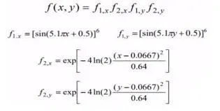
Program for stalagmite function;

function f=stalagmite(input_vector)

x=input_vector(1);
y=input_vector(2);

f1x=(sin(5.1*pi*x+0.5))^6;
f2x=exp((-4)*log(2)*((x-0.0667)^2/0.64));
f1y=(sin(5.1*pi*y+0.5))^6;
f2y=exp((-4)*log(2)*((y-0.0667)^2/0.64));
f=(-1)*f1x*f2x*f1y*f2y;
end

Function program debrief;

Create a function program for a stalagmite function

Assign the input variables to calculate the values in formula

Use the equation of stalagmite function in a program, we will find the f value for the stalagmite function and end the function program.

Program for calculating a global maxima of stalagmite function using Genetic algorithm;

clear all
close all
clc

%defining our search space
x=linspace(0,0.6,150);
y=linspace(0,0.6,150);

%creating a 2Dimensional mesh
[xx yy]=meshgrid(x,y);

% evaluating the stalagmite function
for i=1:length(xx)
    for j=1:length(yy)
        input_vector(1)=xx(i,j);
        input_vector(2)=yy(i,j);
        f(i,j)=stalagmite(input_vector);
    end
end

surf(xx,yy,f)
shading interp

Program debrief;

• Assign the input variable for x and y using linspace command and get a value in matrix.
• Use meshgrid command to get a matrix value of xx and yy.
• Getting the stalagmite function value for x and y values by usimg for loop.
• Using -ve symbol to find the global maxima
• After finding the function value, use surf to plot the values.
• To hide the grid lines use shading interp in the stalagmite plot.

Find global maxima by using Genetic algorithm;

STUDY-1 Unbounded iterations;

clear all
close all
clc

x=linspace(0,0.6,150);
y=linspace(0,0.6,150);


[xx yy]=meshgrid(x,y);


for i=1:length(xx)
    for j=1:length(yy)
        input_vector(1)=xx(i,j);
        input_vector(2)=yy(i,j);
        f(i,j)=stalagmite(input_vector);
    end
end


num_cases=50;

%study1-statistical behaviour
tic

for i=1:num_cases
    [inputs,fopt(i)]=ga(@stalagmite,2);
    xopt(i)=inputs(1);
    yopt(i)=inputs(2);
end
study1_time= toc
figure(1)
subplot(2,1,1)
hold on
surf(x,y,-f)
shading interp
plot3(xopt,yopt,-fopt,'marker','o','markersize',5,'markerfacecolor','r')
title('unbounded inputs')
subplot(2,1,2)
plot(-fopt)
xlabel('iterations')
ylabel('function maximum')
colorbar

program debrief;

STUDY-1 Unbounded conditions.

Assign the num_case value for the limit of ga iterations.

In study 1 – statistical behaviour we get ‘unbounded inputs’ by using the ga syntax of x=ga(fun,vars); and find the xopt,yopt values using ‘for loop’.

Use subplot command to get two plots in a single window

And plot3 command for plot the three values(xopt,yopt,-fopt) in a single plot.

Use plot command to plot the (-fopt) value in the figure window.

Use tic and toc command to calculate the time of getting output of study 1.

STUDY-2 Bounded iterations, ub and lb

clear all
close all
clc

x=linspace(0,0.6,150);
y=linspace(0,0.6,150);


[xx yy]=meshgrid(x,y);


for i=1:length(xx)
    for j=1:length(yy)
        input_vector(1)=xx(i,j);
        input_vector(2)=yy(i,j);
        f(i,j)=stalagmite(input_vector);
    end
end


num_cases=50;

%study2-ststistical behaviour-with upper and lower bound
tic

for i=1:num_cases
    [inputs,fopt(i)]=ga(@stalagmite,2,[],[],[],[],[0;0],[1;1]);
    xopt(i)=inputs(1);
    yopt(i)=inputs(2);
end
study2_time= toc
figure(2)
subplot(2,1,1)
hold on
surf(x,y,-f)
shading interp
plot3(xopt,yopt,-fopt,'marker','o','markersize',5,'markerfacecolor','r')
title('Bounded inputs')
subplot(2,1,2)
plot(-fopt)
xlabel('iterations')
ylabel('function maximum')

program debrief;

Study 2 statistical behaviour with upper and lower bounds we get ‘bounded inputs’ using the ga syntax of x=ga(fun,nvars,A,B,Aeq,Beq,lb,ub); and finding the xopt,yopt values using ‘for loop’.

Similarly like study 1 use subplot, plot3,plot,xlabel,ylabel,tic and toc commands to get output of study 2.

STUDY-3 Bounded iterations, ub and lb with increased population

clear all
close all
clc

x=linspace(0,0.6,150);
y=linspace(0,0.6,150);


[xx yy]=meshgrid(x,y);


for i=1:length(xx)
    for j=1:length(yy)
        input_vector(1)=xx(i,j);
        input_vector(2)=yy(i,j);
        f(i,j)=stalagmite(input_vector);
    end
end


num_cases=50;

%study3-bound calculations with modified population size
tic

options=optimoptions('ga');
options=optimoptions(options,'populationsize',350);

for i=1:num_cases
    [inputs,fopt(i)]=ga(@stalagmite,2,[],[],[],[],[0;0],[1;1],[],[],options);
    xopt(i)=inputs(1);
    yopt(i)=inputs(2);
end
study3_time= toc
figure(3)
subplot(2,1,1)
hold on
surf(x,y,-f)
shading interp
plot3(xopt,yopt,-fopt,'marker','o','markersize',5,'markerfacecolor','r')
title('Bounded inputs with increased population')
subplot(2,1,2)
plot(-fopt)
xlabel('iterations')
ylabel('function maximum')
colorbar

Program debrief;

Study 3- increasing ga iterations we get the global maxima by using ga syntax of x=ga(fun,nvars,A,B,Aeq,Beq,lb,ub,nonlcon,lntcon,options) and find the xopt,yopt values using for loop.

Similarly like study1 and study2 use subplot, plot3,plot,xlabel,ylabel,tic and toc commands to get output of study 3.

Final code;

clear all
close all
clc

x=linspace(0,0.6,150);
y=linspace(0,0.6,150);


[xx yy]=meshgrid(x,y);


for i=1:length(xx)
    for j=1:length(yy)
        input_vector(1)=xx(i,j);
        input_vector(2)=yy(i,j);
        f(i,j)=stalagmite(input_vector);
    end
end
figure(4)
surf(xx,yy,-f)
shading interp
xlabel('x-value')
ylabel('y-value')
colorbar


num_cases=50;

%study1-statistical behaviour
tic

for i=1:num_cases
    [inputs,fopt(i)]=ga(@stalagmite,2);
    xopt(i)=inputs(1);
    yopt(i)=inputs(2);
end
study1_time= toc
figure(1)
subplot(2,1,1)
hold on
surf(x,y,-f)
shading interp
plot3(xopt,yopt,-fopt,'marker','o','markersize',5,'markerfacecolor','r')
title('unbounded inputs')
subplot(2,1,2)
plot(-fopt)
xlabel('iterations')
ylabel('function maximum')
colorbar

%study2-ststistical behaviour-with upper and lower bound
tic

for i=1:num_cases
    [inputs,fopt(i)]=ga(@stalagmite,2,[],[],[],[],[0;0],[1;1]);
    xopt(i)=inputs(1);
    yopt(i)=inputs(2);
end
study2_time= toc
figure(2)
subplot(2,1,1)
hold on
surf(x,y,-f)
shading interp
plot3(xopt,yopt,-fopt,'marker','o','markersize',5,'markerfacecolor','r')
title('Bounded inputs')
subplot(2,1,2)
plot(-fopt)
xlabel('iterations')
ylabel('function maximum')

%study3-bound calculations with modified population size
tic

options=optimoptions('ga');
options=optimoptions(options,'populationsize',350);

for i=1:num_cases
    [inputs,fopt(i)]=ga(@stalagmite,2,[],[],[],[],[0;0],[1;1],[],[],options);
    xopt(i)=inputs(1);
    yopt(i)=inputs(2);
end
study3_time= toc
figure(3)
subplot(2,1,1)
hold on
surf(x,y,-f)
shading interp
plot3(xopt,yopt,-fopt,'marker','o','markersize',5,'markerfacecolor','r')
title('Bounded inputs with increased population')
subplot(2,1,2)
plot(-fopt)
xlabel('iterations')
ylabel('function maximum')

Conclusion;

In MATLAB GA will always gives a minimum value, for finding a maximum value , we can inverse the function, then we will get global maxima of stalagmite function.