Week 7 - Simulation of a 1D Supersonic nozzle flow simulation using Macormack Method
Aim:
To simulate the isentropic flow through a quasi 1D subsonic-supersonic nozzle.
Derive both the conservation and non-conservation forms of the governing equations and sovle them using the MacCormack's technique.
Determine the steady-state temperature distribution for the flow-field variables and investigate the difference between the two forms of governing equations by comparing their solutions.
Theory:
MacCormackMethod:
In computational fluid dynamics, the MacCormack method is a widely used discretization scheme for the numerical solution of hyperbolic partial differential equations.
Algorithm:
Consider the following Hyperbolic Equation:
`(delu)/(delt)+alpha*(delu)/(delx)=0`
The application of MacCormack method to the above equation proceeds in two steps; a predictor step which is followed by a corrector step.
Predictor step:
In the predictor step, a "provisional" value of u at time level n+1 (denoted by `u_i^(bar(n+1))`) is estimated as follows
`u_i^(bar(n+1))=u_i^n-alpha(delt)/(delx)*( u_(i+1)^(bar(n))-u_i^n)`
The above equation is obtained by replacing the spatial and temporal derivatives in the previous first order hyperbolic equation using forward differences.
Corrector Step: In the corrector step, the predicted value `u_i^(bar(n+1))` is corrected according to the equation
`u_i^(bar(n+1))=u_i^(bar(n+1)/2)-alpha(delt)/(delx)*(u_i^(bar(n+1))-u_(i-1)^(bar(n+1)))`
Note that the corrector step uses backward finite difference approximations for spatial derivative. The time-step used in the corrector step is deltat/2 as contrast to delta t in the predictor step.
`u_i^((n+1)/2)=(u_i^(n)+u_i^(bar(n+1)))/2`.
Non Conservative Form
clear all
close all
clc

% Inputs
n=31;
x=linspace(0,3,n);
dx=x(2)-x(1);
gamma=1.4;

% Calculate Initial profiles

rho = 1 - 0.3146 * x;
t = 1 - 0.2314 * x;
v = (0.1+1.09*x).* t.^0.5;

a=1+2.2*(x-1.5).^2;

throat = find(a==1);

M = zeros(1,31);

% plot(a)

% Time steps

nt=500;
dt=0.001;

% outer Time loop

for k=1:nt

    rho_old = rho;
    v_old = v;
    t_old = t;

% predictor method

    for j=2:n-1

        % Common terms

        dvdx = (v(j+1) - v(j))/dx;

        drhodx = (rho(j+1)-rho(j))/dx;

        dtdx = (t(j+1)-t(j))/dx;

        dlogadx = (log(a(j+1))-log(a(j)))/dx;

        % Continuity equation

        drhodt_p(j) = -rho(j)*dvdx - rho(j)*v(j)*dlogadx - v(j)*drhodx;

        % Momentum equation

        dvdt_p(j) = -v(j)*dvdx - (1/gamma)*(dtdx + (t(j)/rho(j))*drhodx);

        % energy equation

        dtdt_p(j) = -v(j)*dtdx - (gamma-1)*t(j)*(dvdx + v(j)*dlogadx);

        % Solution update

        rho(j) = rho(j) + drhodt_p(j) * dt;
        v(j) = v(j) + dvdt_p(j) * dt;
        t(j) = t(j) + dtdt_p(j) * dt;


    end

    % Corrector method

    for j=2:n-1

        dvdx_c = (v(j) - v(j-1))/dx;

        drhodx_c = (rho(j) - rho(j-1))/dx;

        dtdx_c = (t(j) - t(j-1))/dx;

        dlogadx_c = (log(a(j)) - log(a(j-1)))/dx;

        % Continuity equation

        drhodt_c(j) = -rho(j) * dvdx - rho(j) * v(j) * dlogadx_c - v(j) * drhodx_c;

        % Momentum equation

        dvdt_c(j) = -v(j)*dvdx_c - (1/gamma)*(dtdx_c + (t(j)/rho(j))*drhodx_c);

        % energy equation

        dtdt_c(j) = -v(j)*dtdx_c - (gamma-1)*t(j)*(dvdx_c + v(j)*dlogadx_c);

    end
    %     Compute the average time derivative

    drhodt = 0.5*(drhodt_p + dtdt_c);
    dvdt = 0.5*(dvdt_p + dtdt_c);
    dtdt = 0.5*(dtdt_p + dtdt_c);

    residual(k,1) = max(abs(drhodt));
        residual(k,2) = max(abs(dvdt));
        residual(k,3) = max(abs(dtdt));

    %     Final solution update

     for i=2:n-1

        rho(i) = rho_old(i) + drhodt(i) * dt;
        v(i) = v_old(i) + dvdt(i) * dt;
        t(i) = t_old(i) + dtdt(i) * dt;

     end

    % Apply Boundary condition

    %inlet

    v(1) = 2 * v(2) - v(3);

    %outlet

    v(n) = 2 * v(n-1) - v(n-2);
    rho(n) = 2 * rho(n-1) - rho(n-2);
    t(n) = 2 * t(n-1) - t(n-2);

    rho(end) = 2*rho(end-1)-rho(end-2);
        v(1) = 2*v(2)-v(3);
        v(end) = 2*v(end-1)-v(end-2);
        t(end) = 2*t(end-1)-t(end-2);
        M = v/(t(i)^0.5);
        p = rho.*t(i);
        m(k,:) = rho.*a.*v;
        rho_t(k) = rho(throat); v_t(k) = v(throat); t(k) = t(throat);
        p_t(k) = p(throat);
        M_t = M(throat);

%     plot(x,v)
%
%     title(sprintf('Time step is %d',k))
%      pause(0.003)

end

figure(1)
subplot(4,1,1)
plot(x,M)
grid on; ylim([0 4.5]);
ylabel('Mach Number')
title('Flow parameter (non-conservative form of governing equation)')
subplot(4,1,2)
plot(x,p)
grid on;
ylabel('Pressure Ratio')
subplot(4,1,3)
plot(x,rho)
grid on;
ylabel('Density Ratio')
subplot(4,1,4)
plot(x,t)
grid on; ylim([0 1]);
ylabel('Temperature Ratio')
xlabel('X/L')
Conservative form
clear all
close all
clc

% Initializing the domain
L = 3;
nx = 31;
x = linspace(0,L,nx);
dx = x(2)-x(1);
C = 0.5;
nt = 1400;
gamma = 1.4;

% Nozzle area profile
A = 1 + 2.2*(x-1.5).^2;


    % Initial conditions
    rho_0 = zeros(length(x),1);
    T_0 = rho_0;
    V_0 = T_0;
    for i=1:length(x)
        if x(i)>=0 && x(i)<0.5
            rho_0(i) = 1;
            T_0(i) = 1;
        elseif x(i)>=0.5 && x(i)<1.5
            rho_0(i) = 1 - 0.366*(x(i)-0.5);
            T_0(i) = 1 - 0.167*(x(i)-0.5);
        elseif x(i)>=1.5 && x(i)<=3
            rho_0(i) = 0.634 - 0.3879*(x(i)-1.5);
            T_0(i) = 0.833 - 0.3507*(x(i)-1.5);
        end
        V_0(i) = 0.59/(rho_0(i)*A(i));
    end
    throat = find(A==1);
    rho = rho_0;
    T = T_0;
    V = V_0;
    m = zeros(nt,length(x));
    U1 = rho*A;
    U2 = rho*A*V;
    U3 = rho.*(T./(gamma-1) + 0.5*gamma*V.^2).*A;
    rho_t = zeros(nt,1);
    T_t = rho_t;
    V_t = T_t;
    p_t = V_t;
    M_t = p_t;

    residual = zeros(nt,3);

    for k=1:nt
        U1_old = U1; U2_old = U2; U3_old = U3;
        dt = min(C*dx./(T.^0.5 + V));
        F1 = U2;
        F2 = (U2.^2)./U1+((gamma-1)/gamma)*(U3 - 0.5*gamma*(U2.^2)./U1);
        F3 = gamma*U2.*U3./U1 - 0.5*gamma*(gamma-1)*(U2.^3)./(U1.^2);

        % Predictor loop
        for i=2:length(x)-1
            dF1dx = (F1(i+1) - F1(i))/dx;
            dF2dx = (F2(i+1) - F2(i))/dx;
            dF3dx = (F3(i+1) - F3(i))/dx;
            dAdx = (A(i+1) - A(i))/dx;
            J2 = (1/gamma)*rho(i)*T(i)*dAdx;

            dU1dt_p(i) = -dF1dx;
            dU2dt_p(i) = -dF2dx + J2;
            dU3dt_p(i) = -dF3dx;

            % Intermediate update
            U1(i) = U1(i) + dU1dt_p(i)*dt;
            U2(i) = U2(i) + dU2dt_p(i)*dt;
            U3(i) = U3(i) + dU3dt_p(i)*dt;
        end
        rho = U1./A;
        V = U2./U1;
        T = (gamma-1)*((U3./U1) - 0.5*gamma*V.^2);
        F1 = U2;
        F2 = (U2.^2)./U1+((gamma-1)/gamma)*(U3 - 0.5*gamma*(U2.^2)./U1);
        F3 = gamma*U2.*U3./U1 - 0.5*gamma*(gamma-1)*(U2.^3)./(U1.^2);
        % Corrector loop
        for i=2:length(x)-1
            dF1dx = (F1(i) - F1(i-1))/dx;
            dF2dx = (F2(i) - F2(i-1))/dx;
            dF3dx = (F3(i) - F3(i-1))/dx;
            dAdx = (A(i) - A(i-1))/dx;
            J2 = (1/gamma)*rho(i)*T(i)*dAdx;

            dU1dt_c(i) = -dF1dx;
            dU2dt_c(i) = -dF2dx + J2;
            dU3dt_c(i) = -dF3dx;
        end

        % Average of predictor and corrector step
        dU1dt = 0.5*(dU1dt_p + dU1dt_c);
        dU2dt = 0.5*(dU2dt_p + dU2dt_c);
        dU3dt = 0.5*(dU3dt_p + dU3dt_c);
        residual(k,1) = max(abs(dU1dt));
        residual(k,2) = max(abs(dU2dt));
        residual(k,3) = max(abs(dU3dt));

        % Final solution update
        for i=2:length(x)-1
            U1(i) = U1_old(i) + dU1dt(i)*dt;
            U2(i) = U2_old(i) + dU2dt(i)*dt;
            U3(i) = U3_old(i) + dU3dt(i)*dt;
        end

        % Boundary conditions
        U1(1) = rho(1)*A(1);
        U1(end) = 2*U1(end-1) - U1(end-2);
        U2(1) = 2*U2(2) - U2(3);
        U2(end) = 2*U2(end-1) - U2(end-2);
        U3(1) = U1(1)*((T(1)/(gamma-1)) + 0.5*gamma*V(1)^2);
        U3(end) = 2*U3(end-1) - U3(end-2);
        rho = U1./A;
        V = U2./U1;
        T = (gamma-1)*((U3./U1) - 0.5*gamma*V.^2);
        M = V./(T.^0.5);
        p = rho.*T;
%         m(k,:) = rho.*A.*V;
        rho_t(k) = rho(throat); V_t(k) = V(throat); T_t(k) = T(throat);
        p_t(k) = p(throat); M_t(k) = M(throat);
    end
Plots:
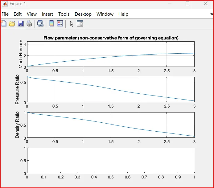
Steady-state distribution of primitive variables inside the nozzle
For the Non Conservative form
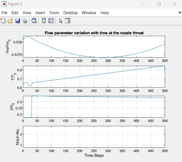
Time-wise variation of the primitive variables
For the Non Conservative form
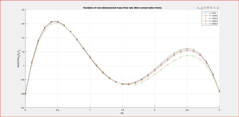
Variation of Mass flow rate distribution inside the nozzle at different time steps during the time-marching process
For the Non Conservative form
Comparison of Normalized mass flow rate distributions of both forms
For the Non Conservative form
Conclusion:
Plot of mach no density and temperature has been generated for the length of nozzle.
Flow parameter at throat is generated WITH TIME.
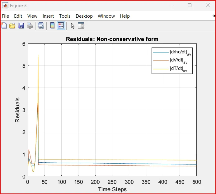
Plot of residuals has been generated.
Mass flow rate throughout the length of the nozzle has been plotted