Week 7 - Simulation of a 1D Super-sonic nozzle flow simulation using Macormack Method
Simulating the isentropic flow through a quasi 1D subsonic-supersonic nozzle
The conservation and non-conservation forms of the governing equations are sovled using the MacCormack's technique as discussed in the videos with reference from Anderson book.
Convergent-Divergent Nozzle:
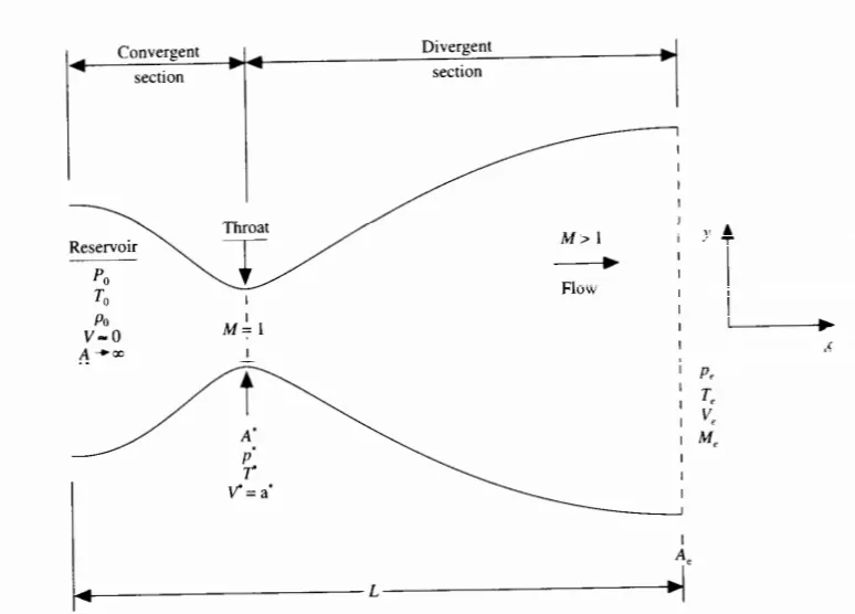
The C-D nozzle picture taken from Anderson book.Here,the steady and isentropic flow through a convergent-divergent nozzle is considered.Here, we assume that flow properties changes only with x-directiont meaning uniform flow properties and called as quasi-one-dimensional flow.
Governing equations to solve this flow will be:
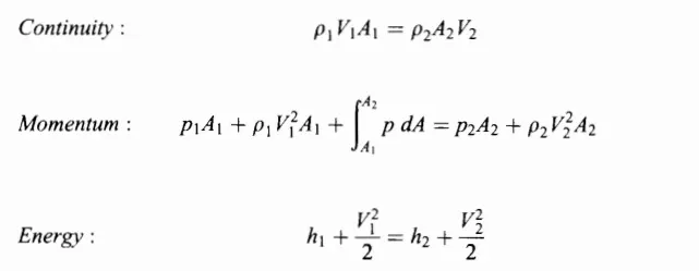
Here `p =rhoRT and h =C_pT`
The Mach number-area relation in the nozzle flow is given as:
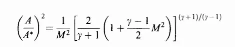
In all the above equations : P =pressure, V=velocity, `rho` = density, T =temperature, M =mach number, A =area,`gamma` =1.4, and '*' value indicates throat values.
MacCormack's technique:
In this technique, we use time marching finte difference CFD solution for Quasi- 1D nozzle flow.This discretisation scheme is useld mostly for numerical solution of hyperbolic pde's.The governing quations are presented in pde forms for time marching with finite differencing methods accordingly in predictor and corrector step.
We non dimensional all the varibles in this method as follows:
`T^' = T/T_o; rho^' =rho/rho_o;V^' =V/a_o;`
`t^' =t/({L/a_o}); A^' =A/A^star`
`a_o=sqrt(gammaRT_o) ; x' =x/L;`
'o' indicates reservoir properties, t is time, L is length of nozzle,`a_o` is dimensionaless velocity.
With this parameters we have governing equations for the nozzle flow CFD calculations from Anderson book are as follows:
Non conservative form:
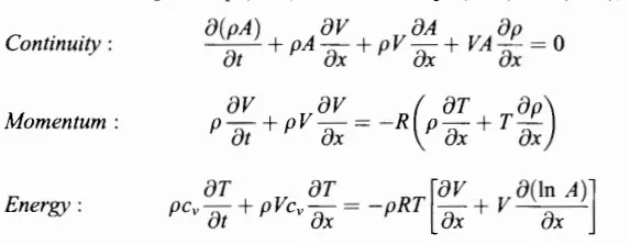
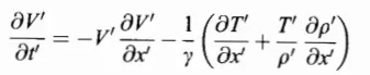
These equation can be re written in non -dimensional form as :
Continuity equation as

Momentum equation as
Energy equation as:

Hence solving equations for density, velocity and temperature
Conservative form:
Continuity equation:
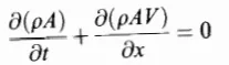
Momentum equation:

Energy equation:

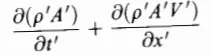
Non dimensional form of the above equation will be:
 = 0
= 0


Now to further simplify this equations to solve , some elements are defined as : Solution vector U; Flux vector F and source term J;
Step by step procedure followed for both methods:
Problem formulation: Simulate the isentropic flow through a quasi 1D subsonic-supersonic nozzle and derive both the conservation and non-conservation forms of the governing equations and sovle them using the MacCormack's technique.
Geometry: Length of nozzle is taken as L(L=3) since it is 1D quasi dimensional. Also,Area will be
`A = 1+2.2(x-1.5)^2`
Throat = (n+1)/2;
Mesh: The length domain is divided in to number of elements as n(we take n=31 ) for initial study.
Numerical Scheme: As mentioned , MacCormack method is used with pde and finite differencing.We use forward and back ward differencing in predictor and correcter methods accordingly for solving all the primitive variable in this flow field.
`Deltat = C(Delta x)/(a+v)`
C =courant number (0.5 here) and a =`sqrtT`(speed of sound)
`Delta x =x(2)-x(1) or L/(n-1)` and v is flow velocity
This is local time marching approach and hence we use minimum value of `Delta t` for obtaining correct steady state and noted as "dt"
Flow chart of our codes with MacCormack method will be:
- Initial and Boundary conditions
- Initial profiles (`rho,`T,V,a) and throat
- Time loop
- Predictor Method (FDS)
- Solution update
- Corrector Method(BDS)
- Solution update
- Time derivatives average
- Final solution update
Here the methodology is same for both conservative and non conservative methods but the initial profiles used and variable solved for governing equations are different.They are as follows:
Non conservative form:
Initial profiles or conditions:
`rho =1-0.3146*x`
`T = 1-0.2314*x`
`V = (0.1+1.09*x)*sqrt(T)`
Boundary conditions:
At Inlet : `rho(1) =1; T(1) =1;V_1=2V_2-V_3`
At outlet : `rho(n) =2*rho(n-1)-rho(n-2);T(n) =2*T(n-1)-T(n-2);V(n) =2*V(n-1)-V(n-2);`
Conservative form:
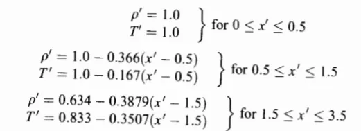
Initial profiles or conditions:
and
`V^' =U_2/(rho^'*A^') =0.59/(rho^'*A^')`
U is solution vector and these vectors are used in place of primite variables discussed in anderson book as:
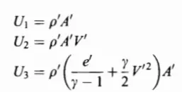
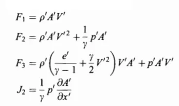
U1,U2,U3 are solution vectors, F1,F2,F3 are flux vectors and J2 is source term. e is temperature;
Here,
`rho^' = U_1/A^';V^' = U_2/U_1; P^' =rho^'*T^'`
`T^' = (gamma-1)(U_3/U_2-gamma/2(V^('2)))`
Using this non dimensional terms we have governing equations re written as :
`(delU_1)/(dt^')=-(delF_1)/(dx^')`
`(delU_2)/(dt^')=-(delF_2)/(dx^')+J_2`
`(delU_3)/(dt^')=-(delF_3)/(dx^')`
Since since we update solution with flux vectors and we write flux vectors in terms of solution vectors as:
`F_1 =U_2`
`F_2 =(U_2)^2/U_1+(gamma-1)/gamma*(U_3-gamma/2*(U_2)^2/U_1)`
`F_3=gamma(U_2*U_3)/U_1+((gamma-1)*gamma)/2*((U_3)/U_1)^2`
`J_2 =(gamma-1)/gamma*(U_3-gamma/2*(U_2)^2/U_1)*(del(lnA^'))/(delx^')`
Hence these terms are used for preventing the repeating of errors while running the solution with time marching method.
Boundary conditions:
At inlet :
`U_1 (1) =rho^'(1)*A^'(1)`
`U_2 (1) =2*U_2(2)-U_2(3)`
`U_3(1) = (T^'/(gamma-1)+gamma/2(V^')^2)`
`rho(1) =1`
`T(1) =1`
At outlet:
`U_1(n) = 2U_1(n-1)-U_1(n-2)`
`U_2(n) = 2U_2(n-1)-U_2(n-2)`
`U_3(n) = 2U_3(n-1)-U_3(n-2)`
Hence for the both the methods with the above governing equations, initial and boundary conditiond the code is run for 1400 steps and the solution variables are updated and plotted according as required in the problem.
Matlab code:
Non Conservative form:
clear all
close all
clc
%inputs
n =31;
x =linspace(0,3,n);
dx = x(2)-x(1);
gamma =1.4;
%calculate initial profiles
rho = 1-(0.3146*x);
t = 1-(0.2314*x); %temperature
v =(0.1+1.09*x).*sqrt(t);
%area
a =1+2.2*(x-1.5).^2;
throat = (n+1)/2;
%time steps
nt =1400;
C =0.5;
dt = min(C*(dx./(sqrt(t)+v)));
%dt =0.01;
%outer time loop
for k =1:nt
    rho_old =rho;
    v_old =v;
    t_old =t;
    %predictor method


    for j =2:n-1
        %drho_dt_p =(-rho(j)*(v(j+1)-v(j))/dx)-(rho(j)*v(j)*(log(a(j+1)-log(a(j)))/dx)-(v(j)*((rho(j+1)-rho(j))/dx)
        dvdx = (v(j+1)-v(j))/dx;
        drhodx = (rho(j+1)-rho(j))/dx;
        dtdx = (t(j+1)-t(j))/dx;
        %dlog_a_dx
        dlogadx = (log(a(j+1))-log(a(j)))/dx;
        %continuity equation
        drhodt_p(j) = -rho(j)*dvdx - rho(j)*v(j)*dlogadx -v(j)*drhodx;
        %momentum equation
        dvdt_p(j) = -v(j)*dvdx-(1/gamma)*(dtdx+(t(j)/rho(j))*drhodx);
        %energy equation
        dtdt_p(j) = -v(j)*dtdx -(gamma-1)*t(j)*(dvdx+v(j)*dlogadx);
        %solution update
     rho(j) =rho(j)+drhodt_p(j)*dt;
    v(j) =v(j)+dvdt_p(j)*dt;
    t(j) = t(j)+dtdt_p(j)*dt;
    end
    %correcter method
     for j =2:n-1
        %drho_dt_p =(-rho(j)*(v(j+1)-v(j))/dx)-(rho(j)*v(j)*(log(a(j+1)-log(a(j)))/dx)-(v(j)*((rho(j+1)-rho(j))/dx)
        dvdx = (v(j)-v(j-1))/dx;
        drhodx = (rho(j)-rho(j-1))/dx;
        dtdx = (t(j)-t(j-1))/dx;
        %dlog_a_dx
        dlogadx = (log(a(j))-log(a(j-1)))/dx;
        %continuity equation
        drhodt_c(j) = -rho(j)*dvdx - rho(j)*v(j)*dlogadx -v(j)*drhodx;
        %momentum equation
        dvdt_c(j) = -v(j)*dvdx-(1/gamma)*(dtdx+(t(j)/rho(j))*drhodx);
        %energy equation
        dtdt_c(j) = -v(j)*dtdx -(gamma-1)*t(j)*(dvdx+v(j)*dlogadx);

     end
    %compute the average time derivative
    drhodt =0.5*(drhodt_p+drhodt_c);
    dvdt =0.5*(dvdt_p+dvdt_c);
    dtdt =0.5*(dtdt_p+dtdt_c);
    %final solution update
    for i =2:n-1
    rho(i) =rho_old(i)+drhodt(i)*dt;
    v(i) =v_old(i)+dvdt(i)*dt;
    t(i)= t_old(i)+dtdt(i)*dt;
    end
    %apply boundary bc
    %inlet
    v(1) =2*v(2)-v(3);
    %outlet
    rho(n) =2*rho(n-1)-rho(n-2);
    v(n) =2*v(n-1)-v(n-2);
    t(n) =2*t(n-1)-t(n-2);
    %flow parameters
    p =rho.*t;
    M =  v./sqrt(t);
    mass_flow_rate_nc = rho.*a.*v;

    %throat
    rho_t(k) = rho(throat);
    t_t(k) =t(throat);
    p_t(k) = p(throat);
    mass_flow_rate_t_nc(k) =mass_flow_rate_nc(throat);
    M_t(k) =M(throat);
    v_t(k) =v(throat);
    %mass flow rate at different time step
    % Variation of Mass flow rate distribution inside the nozzle at different time steps during the time-marching process
    figure(1)
        hold on

    if k == 1
        plot (x,mass_flow_rate_nc,'b')
        hold on
        grid on

    elseif k ==50
        plot (x,mass_flow_rate_nc,'g')
        hold  on

    elseif k ==100
        plot (x,mass_flow_rate_nc, 'r')
        hold on

    elseif k ==200
        plot (x,mass_flow_rate_nc,'c')
        hold on
         elseif k ==400
        plot (x,mass_flow_rate_nc,'y')
        hold on


    elseif k ==800
        plot (x,mass_flow_rate_nc,'m')
        hold on
        elseif k ==1400
        plot (x,mass_flow_rate_nc,'p')


       xlabel ('length of nozzle')
        ylabel ( 'mass flow rate')
        title( ' Mass flow rate at time steps for Non conservative')
       legend ('1Deltat','50 Deltat','100Deltat','200Deltaat','400Deltat','800Deltat','1400Deltat')

    end
end
%Steady-state distribution of primitive variables inside the nozzle
figure(2)
%density
subplot(4,1,1)
plot(x,rho,'b','linewidth',2)
xlabel('nozzle non dimensional length')
ylabel ('density(rho/rho_0)')
title('Steady-state distribution of primitive variables')
%velocity
subplot(4,1,2)
plot(x,v,'r','linewidth',2)
xlabel('nozzle non dimensional length')
ylabel ('velocity(v/v_0)')

%temperature
subplot(4,1,3)
plot(x,t,'g','linewidth',2)
xlabel('nozzle non dimensional length')
ylabel ('temperature(T/T_0')

%pressure
subplot(4,1,4)
plot(x,p,'m','linewidth',2)
xlabel('nozzle non dimensional length')
ylabel ('pressure(P/P_0)')


figure(3)
%flow field at throat
%Time-wise variation of the primitive variables
subplot(4,1,1)
plot(1:nt,rho_t,'b','linewidth',2)
xlabel('Time steps')
ylabel('density(rho/rho_0)')
title('Time-wise variation of the primitive variables')

subplot(4,1,2)
plot(1:nt,v_t,'r','linewidth',2)
xlabel('Time steps')
ylabel('Velocity(v/v_o)')
subplot(4,1,3)
plot(1:nt,t_t,'g','linewidth',2)
xlabel('Time steps')
ylabel('Temperature(t/t_o)')
subplot(4,1,4)
plot(1:nt,M_t,'m','linewidth',2)
xlabel('Time steps')
ylabel('Mach(M)')
%Normalized mass flow rate distribution
figure(4)
plot(x,mass_flow_rate_nc,'b','linewidth',2)
xlabel ('Non dimensional nozzle lenth(x/L)')
ylabel('rho*a*v/rho_0*a_0*v_0')
title('Normalized mass flow rate distribution along Nozzle')
figure(5)
plot(1:nt,mass_flow_rate_t_nc,'r','linewidth',2)
xlabel ('Time steps')
ylabel('rho*a*v/rho_0*a_0*v_0')
title('Normalized mass flow rate distribution in time marching process')
Conservative form:
clear all
close all
clc
%inputs
n =31;
L=3;
x =linspace(0,L,n);
dx = L/(n-1);
gamma =1.4;
%area
a =1+2.2*(x-1.5).^2;
throat = (n+1)/2;

  %calculate initial profiles
      % rho = 1-0.3146*x;
%T = 1-0.2314*x; %temperature


for i =1:n
    if x(i)>=0 && x(i)<=0.5
        rho(i) =1;
        T(i) =1;
    elseif x(i)>=0.5 && x(i)<=1.5
        rho(i) =1-(0.366*(x(i)-0.5));
        T(i) =1-(0.167*(x(i)-0.5));
    elseif x(i)>=1.5 && x(i)<=3
        rho(i) =0.634-(0.3879*(x(i)-1.5));
        T(i) =0.833-(0.3507*(x(i)-1.5));
    end
end
     v =0.59./(rho.*a);
p =rho.*T ;

%solution vectors
U1 =rho.*a;
U2 = rho.*a.*v;
U3 = rho.*(T./(gamma-1)+(gamma/2)*(v.^2)).*a;


%time steps
C = 0.5;
 delt = C.*(dx./(sqrt(T)+v));%7.75
 dt = min(delt);
nt =1400;
%dt =0.0267;
error =1e-4;
%initialization
p_init =p;
v_init=v;
%rho_init =rho;
%T_init=T;
U1_init =U1;
U2_init =U2;
U3_init =U3;

%outer time loop
for k =1:nt
    U1_old =U1;
    U2_old =U2;
    U3_old =U3;
    %flux vectors
F1 =U2;
F2 =((U2.^2)./U1)+((gamma-1)/gamma)*(U3-(0.5*gamma*U2.^2)./U1);
F3 = ((gamma*U2.*U3)./U1)-((0.5*gamma*(gamma-1)*U2.^3)./(U1.^2));

    %predictor method


    for j =2:n-1

        dF1dx = (F1(j+1)-F1(j))/dx;
        dF2dx = (F2(j+1)-F2(j))/dx;
        dF3dx = (F3(j+1)-F3(j))/dx;
        %dlog_a_dx
        dadx =((a(j+1))-(a(j)))/dx;

        %continuity equation
        dU1dt_p(j) = -dF1dx;
        %j2 term
         J2(j) = (1/gamma)*rho(j).*T(j).*dadx;
        %momentum equation
        dU2dt_p(j) = -dF2dx+J2(j);
        %energy equation
        dU3dt_p(j) = -dF3dx;
        %solution update
       U1(j) =U1(j)+dU1dt_p(j)*dt ;
    U2(j) =U2(j)+dU2dt_p(j)*dt;
    U3(j) = U3(j)+dU3dt_p(j)*dt;
    end
    %updated flow variables
rho =U1./a;
     v = U2./U1;
     T = (gamma-1)*(U3./U1 - (gamma/2)*v.^2);
    %upated flux vectors
    F1 =U2;
F2 =((U2.^2)./U1)+((gamma-1)/gamma)*(U3-(0.5*gamma*U2.^2)./U1);
F3 = ((gamma*U2.*U3)./U1)-((0.5*gamma*(gamma-1)*U2.^3)./(U1.^2));


%correcter method
     for j =2:n-1

        dF1dx = (F1(j)-F1(j-1))/dx;
        dF2dx = (F2(j)-F2(j-1))/dx;
        dF3dx = (F3(j)-F3(j-1))/dx;
        %dlog_a_dx
        dadx = ((a(j))-(a(j-1)))/dx;

        %continuity equation

        dU1dt_c(j) = -dF1dx;
        %j2 term
         J2(j) = (1/gamma)*rho(j)*T(j)*dadx;
        %momentum equation
        dU2dt_c(j) = -dF2dx+J2(j);
        %energy equation
        dU3dt_c(j) = -dF3dx;

     end
    %compute the average time derivative
    dU1dt =0.5*(dU1dt_p+dU1dt_c);
    dU2dt =0.5*(dU2dt_p+dU2dt_c);
    dU3dt =0.5*(dU3dt_p+dU3dt_c);
    %final solution update
    for m =2:n-1
    U1(m) =U1_old(m)+dU1dt(m)*dt;
    U2(m) =U2_old(m)+dU2dt(m)*dt;
    U3(m)= U3_old(m)+dU3dt(m)*dt;
    end
    %apply boundary bc
    %inlet
 rho(1) =1;
  T(1) =1;
  U1(1) =rho(1)*a(1);
 U2(1) =2 *U2(2)-U2(3);
 U3(1) = U1(1)*((T(1)/(gamma-1))+((gamma/2)*((U2(1)/U1(1))^2)));
    %outlet
    U1(n) =2*U1(n-1)-U1(n-2);
    U2(n) =2*U2(n-1)-U2(n-2);
    U3(n) =2*U3(n-1)-U3(n-2);
    %update flow properties
     rho =U1./a;
     v = U2./U1;
     T = (gamma-1)*(U3./U1 - (gamma/2)*v.^2);
        p =rho.*T;
    M =  v./sqrt(T);
    mass_flow_rate = rho.*a.*v;

    %throat
    rho_t(k) = rho(throat);
    T_t(k) =T(throat);
    p_t(k) = p(throat);
    mass_flow_rate_t(k) =mass_flow_rate(throat);
    M_t(k) =M(throat);
    v_t(k) =v(throat);

   %mass flow rate at different time step
    % Variation of Mass flow rate distribution inside the nozzle at different time steps during the time-marching process
    figure(1)
        hold on

    if k == 1
        plot (x,mass_flow_rate,'b')
        hold on


    elseif k ==50
        plot (x,mass_flow_rate,'g')
        hold  on

    elseif k ==100
        plot (x,mass_flow_rate, 'r')
        hold on

    elseif k ==200
        plot (x,mass_flow_rate,'c')
        hold on
         elseif k ==400
        plot (x,mass_flow_rate,'y')
        hold on


    elseif k ==800
        plot (x,mass_flow_rate,'m')
        hold on
        elseif k ==1400
        plot (x,mass_flow_rate,'p')


       xlabel ('length of nozzle')
        ylabel ( 'mass flow rate')
        title( ' Mass flow rate at time steps for Non conservative')
       legend ('1Deltat','50 Deltat','100Deltat','200Deltaat','400Deltat','800Deltat','1400Deltat')


    end

end
%Steady-state distribution of primitive variables inside the nozzle
figure(2)
%density
subplot(4,1,1)
plot(x,rho,'b','linewidth',2)
xlabel('nozzle non dimensional length')
ylabel ('density(rho/rho_0)')
title('Steady-state distribution of primitive variables')
%velocity
subplot(4,1,2)
plot(x,v,'r','linewidth',2)
xlabel('nozzle non dimensional length')
ylabel ('velocity(v/v_0)')

%temperature
subplot(4,1,3)
plot(x,T,'g','linewidth',2)
xlabel('nozzle non dimensional length')
ylabel ('temperature(T/T_0')

%pressure
subplot(4,1,4)
plot(x,p,'m','linewidth',2)
xlabel('nozzle non dimensional length')
ylabel ('pressure(P/P_0)')


figure(3)
%flow field at throat
%Time-wise variation of the primitive variables
subplot(4,1,1)
plot(1:nt,rho_t,'b','linewidth',2)
xlabel('Time steps')
ylabel('density(rho/rho_0)')
title('Time-wise variation of the primitive variables')

subplot(4,1,2)
plot(1:nt,v_t,'r','linewidth',2)
xlabel('Time steps')
ylabel('Velocity(v/v_o)')
subplot(4,1,3)
plot(1:nt,T_t,'g','linewidth',2)
xlabel('Time steps')
ylabel('Temperature(t/t_o)')
subplot(4,1,4)
plot(1:nt,M_t,'m','linewidth',2)
xlabel('Time steps')
ylabel('Mach(M)')
%Normalized mass flow rate distribution
figure(4)
plot(x,mass_flow_rate,'b','linewidth',2)
xlabel ('Non dimensional nozzle lenth(x/L)')
ylabel('rho*a*v/rho_0*a_0*v_0')
title('Normalized mass flow rate distribution along Nozzle')
figure(5)
plot(1:nt,mass_flow_rate_t,'r','linewidth',2)
xlabel ('Time steps')
ylabel('rho*a*v/rho_0*a_0*v_0')
title('Normalized mass flow rate distribution in time marching process')
Results and observations:
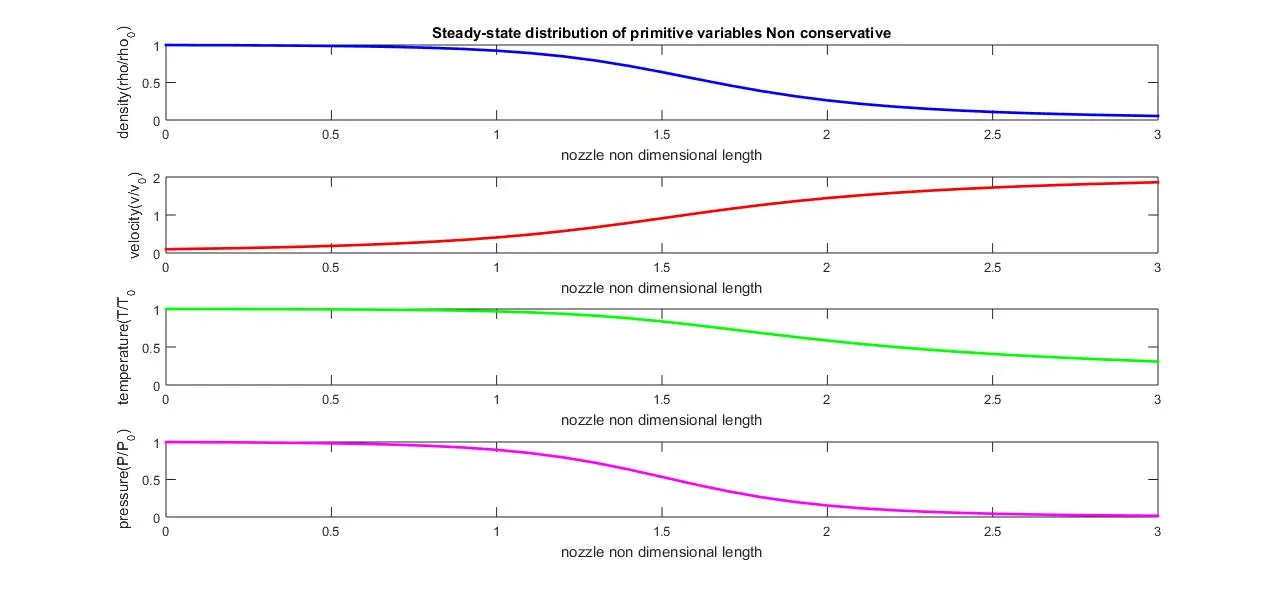
1.Steady-state distribution of primitive variables inside the nozzle
Non conservative form:
Conservative form:
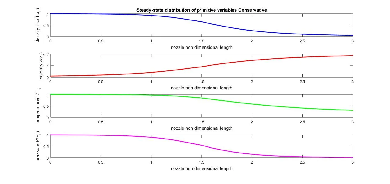
In the challenge , it is asked to determine the steady-state temperature distribution for the flow-field variables. Here we have plots for both form for all primitive variables in both conservative and non conservative forms.
From the investigation of steady state distribution , we have observed that there is gradual decrease in temperature along the length of nozzle along with pressure and density.
Since it is convergent divergent nozzle, there is increase in velocity and the mach number reaches 1 at nozzle throat(choked condition) and the flow becomes supersonic in divergent section. The results obtained with both conservative and non conservative forms are same and no major difference noticed.
2. Time-wise variation of the primitive variables:
Non conservative form:
Conservative form:
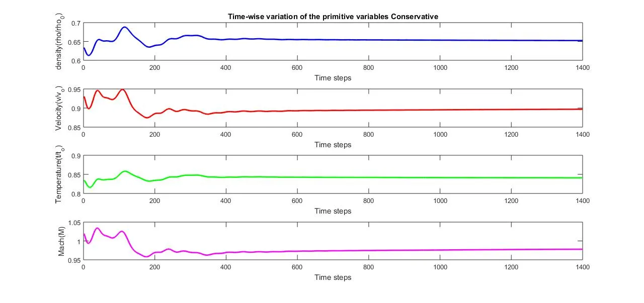
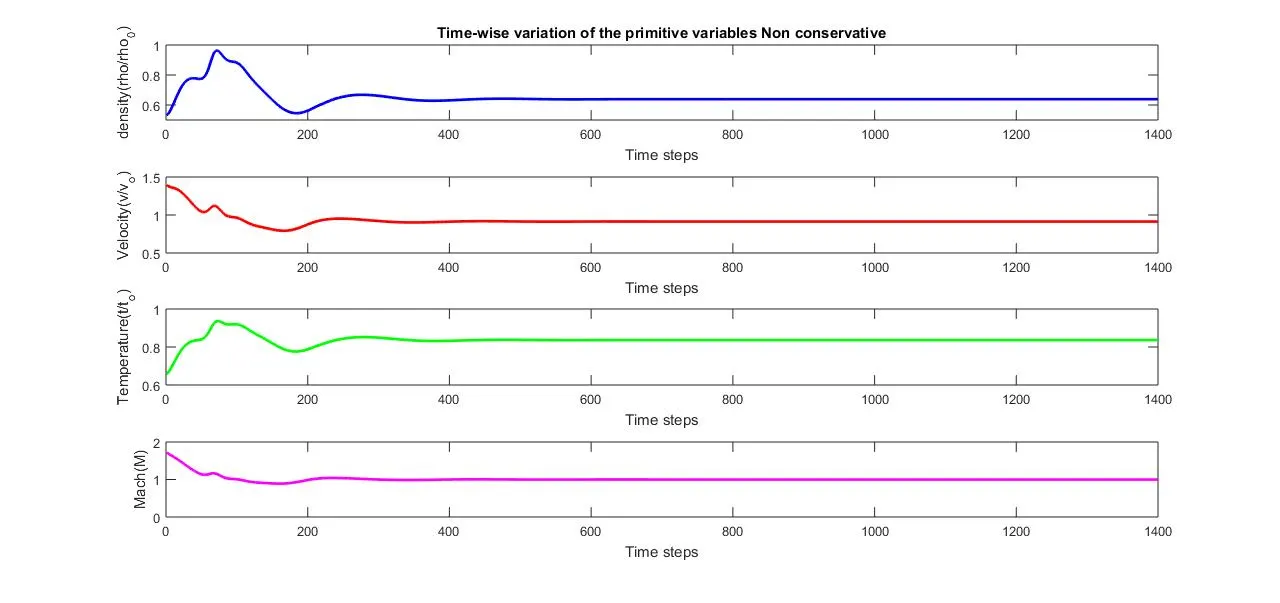
The codes for both the methods is run for 1400 time steps with courant number 0.5 and time step size dt as mention in anderson book.The results obtained are as above.
We observe that all the variables become steady after 800 time steps and the convergence occurs accordingly. There is no much difference between both the forms except the oscillations due to different initial profiles and boundary conditions.
The above time plots are taken at the throat section where n=16; and variation with respect to time is plotted.(just for reference to anderson book, this throat values are taken)
3. Variation of Mass flow rate distribution inside the nozzle at different time steps during the time-marching process
Non conservative form:
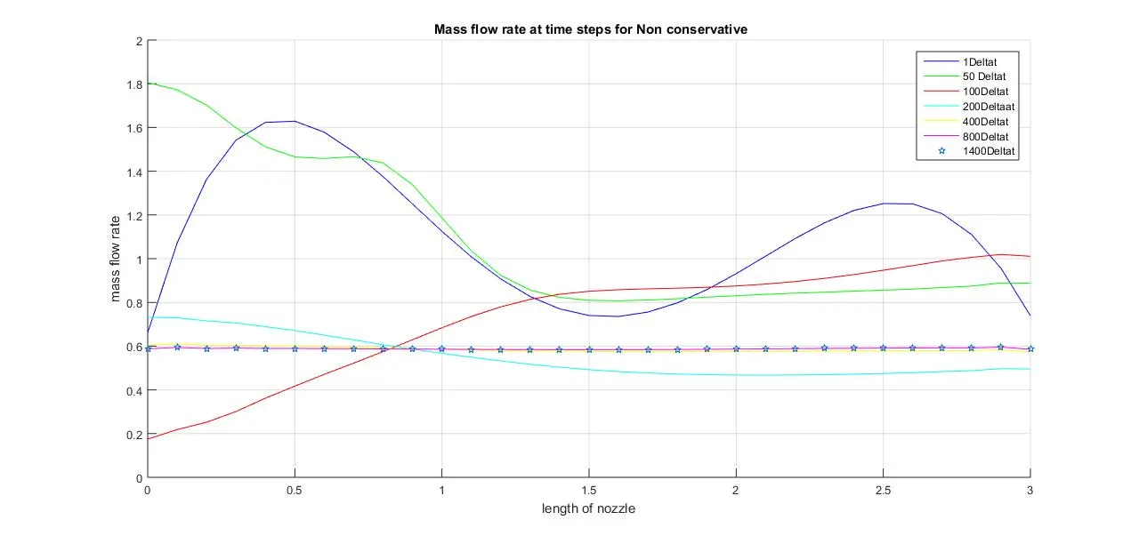
Initial curve at 1 delta t is resultant of product of just rho and v.After some time steps(50) the mass flow distribution changes slightly.After 100 time steps there is radical change and the mass flow distribution has fluctation along the nozzle length andslowly starts settling down at 200 time steps and observed that it settles down with uniform rate from 400 steps and above.
Conservative form:
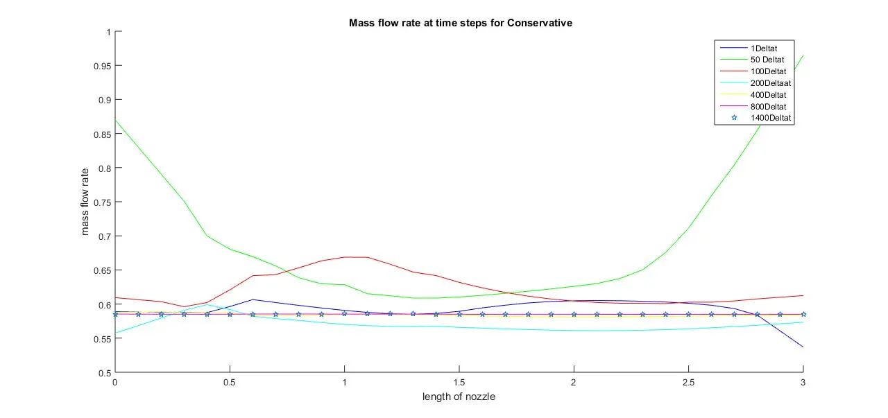
As mentioned in non conservative at 1 deltat the initial condition product is the curve obtaied and the distribution deviaties for 50 time steps and at 100 time steps the distribution is "humped" .But slowly the mass fow rate starts to slettle down at 200 time steps becoming constant and after 400 time steps the mass flow distribution is almost constant and is equal tot the value of 0.579.
The above plots are for Instantaneous distribution of non dimensional mass flow rate along the lenth of nozzle at different time steps during time marching approach to the steady state.
In both the plots,the conservative mass flow steady state distribution is close to analytical value due to presumed inital conditions in the form of flux and solution vectors .
4. Comparison of Normalized mass flow rate distributions of both forms
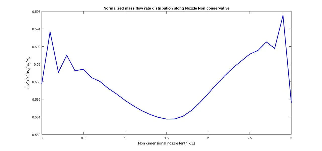
Non conservative form:
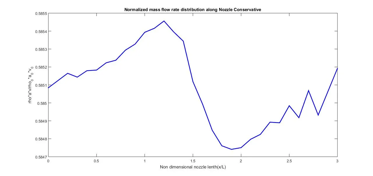
Conservative form:
Code for plotting both forms mass flow distribution :
Here the values from non conservation form are retained in the work space of matlab and conservative form code is run and thus plots are done accordingly alon the nozzle length and for the time steps in time marching approach.
figure(1)
plot(x,mass_flow_rate,'linewidth',2);
hold on;
plot(x,mass_flow_rate_nc,'linewidth',2);
hold off;
xlabel ('Non dimensional nozzle lenth(x/L)')
ylabel('rho*a*v/rho_0*a_0*v_0')
title('Normalized mass flow rate distribution along Nozzle')
legend('Conservative form','Non conservative form')
figure(2)
plot(1:nt,mass_flow_rate_t,'linewidth',2);
hold on;
plot(1:nt,mass_flow_rate_t_nc,'linewidth',2);
hold off;
xlabel ('Time steps)')
ylabel('rho*a*v/rho_0*a_0*v_0')
title('Normalized mass flow rate distribution along Nozzle')
legend('Conservative form','Non conservative form')
Mass flow rate distribution along the nozzle length:
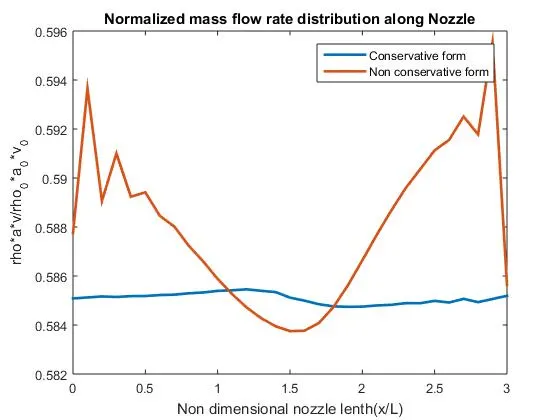
A detailed plot for comparison of the steady state mass flow variation using non conservative and non conservative governing equations.
Here the conservation form on the whole length gives more constant distribution closer to analytical solution of `rho^'A^'V^ ' =0.579`(at throat even non conservative is closer to analytical value due to choking of throat).Hence we can say that in conservation form , the mass in the flow field is preserved than non conservative form. This is due to the dependant variables are primitive in non conservation and secondary varibales result (as mass flow itself is dependant variable here)in conservation form.
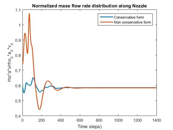
Similarly, the instantaneous mass flow distribution is plotted for the time steps calculated at 1400 time steps. And the steady state acheived almost at 600 time steps.
GRID INDEPENDENCE:
The grid independence is check by monitoring the values of primitive variables at throat for different meshes(grids) (n=31,61).
| `rho^star/rho_0` | `T^star/T_0` | `P^star/P_0` | Mass flow rate | M | |
| Analytical solution values | 0.634 | 0.833 | 0.528 | 0.579 | 1.000 |
| Non conservative form(n=31) | 0.6387 | 0.8365 | 0.5342 | 0.5838 | 0.9994 |
| Conservative form (n=31) | 0.6524 | 0.8410 | 0.5487 | 0.5851 | 0.9780 |
| Non conservative form(n=61) | 0.6377 | 0.8354 | 0.5327 | 0.5827 | 0.9998 |
| conservative form (n=61) | 0.6391 | 0.8355 | 0.5340 | 0.5829 | 0.9979 |
All the values are compared with the analytical or exact solution,Here we observe the non conservative form values are distinctly closer to analytical values.
Also the values at n= 31, 61 tshows the grid independence for both the form with quite change in third order value.Hence by doubling the grid, the valuesare closer to analytical values than n=31 points.But the grid independency starts with n=31 poits as mentioned in anderson book.
Overall Summary:
1.From the the plots above, the conservation form is good at mass conservation .
2.The accuracy is same in both the forms,but non conservation primitive variable values are more accurate and close to analytical values and conservative flux vectors are more accurate than its primitive variables.
3.Conservation form requires more time compared to Non conservation form
4.Both conservation and non conservation forms are grid independant
5.Both the forms are almost similar in results for steady state distribution along the nozzle length for its primitive varibales and attain steady state above 600 steps.