Week 7 - Simulation of a 1D Super-sonic nozzle flow simulation using Macormack Method
INTRODUCTION
The flow through a convergent-divergent nozzle is simulated using the MacCormack's method. The flow through the nozzle is assumed to be a one-dimensional flow. This is an approximation since the flow through a nozzle is 2D in nature, but the 1D approximation is very reasonable in the engineering standpoint since the variation of properties normal to the axis of the nozzle is negligible since the property variations that are relevant in the engineering point of view is along the axis of the nozzle.
The importance of the 1D approximation is the simplicity it affords in rapid calculations from an engineering standpoint. There are many ways in which the supersonic nozzle through a convergent-divergent nozzle can be solved. In this study, we are using the famous MacCormack's method is a widely used discretization scheme used for the solution of hyperbolic PDEs. This second-order finite difference method was introduced by Robert W. MacCormack in 1969.
In this study, the PDEs in the conservative and the non-conservative form are solved. The code for implementing the MacCormack's method was implemented in Matlab and the results are also visualized using Matlab. The governing equations, initial and boundary conditions were taken from the book "Computational Fluid Dynamics The Basics with Application" by John D. Anderson.
OBJECTIVE
The objective of this study is to implement the MacCormack's method in the simulation of a 1D super-sonic nozzle flow and to carry out a grid independence test.
MATHEMATICAL MODELLING
The governing equations of the 1D supersonic nozzle flow can be modeled in two mathematically equivalent forms the conservative and the non-conservative forms.
The primitive variables are non dimensionalized for easy calculations. The non-conservative form of the continuity, momentum, energy equation for quasi-one-dimensional nozzle flow is shown below:
The continuity equation in the non-conservative form : `\frac{\partial \rho^{\prime}}{\partial t^{\prime}}=-\rho^{\prime} \frac{\partial V^{\prime}}{\partial x^{\prime}}-\rho^{\prime} V^{\prime} \frac{\partial\ln A^{\prime}}{\partial x^{\prime}}-V^{\prime} \frac{\partial \rho^{\prime}}{\partial x^{\prime}}`
The momentum equation in the non-conservative form : `\frac{\partial V^{\prime}}{\partial t^{\prime}}=-V^{\prime} \frac{\partial V^{\prime}}{\partial x^{\prime}}-\frac{1}{\gamma}(\frac{\partial T^{\prime}}{\partial x^{\prime}}+\frac{T^{\prime}}{\rho^{\prime}} \frac{\partial \rho^{\prime}}{\partial x^{\prime}})`
The energy equation in the non-conservative form : `\frac{\partial T^{\prime}}{\partial t^{\prime}}=-V^{\prime} \frac{\partial T^{\prime}}{\partial x^{\prime}}-(\gamma-1) T^{\prime}[\frac{\partial V^{\prime}}{\partial x^{\prime}}+V^{\prime} \frac{\partial(\ln A^{\prime})}{\partial x^{\prime}}]`
The finite-difference equations for the non-conservative form of the governing equation are shown below:
`(\frac{\partial \rho}{\partial t})_{i}^{t}=-\rho_{i}^{t} \frac{V_{i+1}^{t}-V_{i}^{t}}{\Delta x}-\rho_{i}^{t} V_{i}^{t} \frac{\ln A_{i+1}-\ln A_{i}}{\Delta x}-V_{i}^{t} \frac{\rho_{i+1}^{t}-\rho_{i}^{t}}{\Delta x}`
`(\frac{\partial V}{\partial t})_{i}^{t}=-V_{i}^{t} \frac{V_{i+1}^{t}-V_{i}^{t}}{\Delta x}-\frac{1}{\gamma}(\frac{T_{i+1}^{t}-T_{i}^{t}}{\Delta x}+\frac{T_{i}^{t}}{\rho_{i}^{t}} \frac{\rho_{i+1}^{t}-\rho_{i}^{t}}{\Delta x})`
`(\frac{\partial T}{\partial t})_{i}^{t}=-V_{i}^{t} \frac{T_{i+1}^{t}-T_{i}^{t}}{\Delta x}-(\gamma-1) T_{i}^{t}(\frac{V_{i+1}^{t}-V_{i}^{t}}{\Delta x}+V_{i}^{t} \frac{\ln A_{i+1}-\ln A_{i}}{\Delta x})`
The predicted values of `\rho`, `V` and `T` can be calculated using the formula shown below, where the barred quantities represents the predicted values.
`\bar{\rho}_{i}^{t+\Delta t}=\rho_{i}^{t}+(\frac{\partial \rho}{\partial t})_{i}^{t} \Delta t`
`\bar{V}_{i}^{t+\Delta t}=V_{i}^{t}+(\frac{\partial V}{\partial t})_{i}^{t} \Delta t`
`\bar{T}_{i}^{t+\Delta t}=T_{i}^{t}+(\frac{\partial T}{\partial t})_{i}^{t} \Delta t`
For the corrector step, the partial difference equations are evaluated using the backward difference formula, which is shown below:
`\begin{aligned} \left(\frac{\overline{\partial \rho}}{\partial t}\right)_{i}^{t+\Delta t}=&-\bar{\rho}_{i}^{t+\Delta t} \frac{\bar{V}_{i}^{t+\Delta t}-\bar{V}_{i-1}^{t+\Delta t}}{\Delta x}-\bar{\rho}_{i}^{t+\Delta t} \bar{V}_{i}^{t+\Delta t} \frac{\ln A_{i}-\ln A_{i-1}}{\Delta x} &-\bar{V}_{i}^{t+\Delta t} \frac{\bar{\rho}_{i}^{t+\Delta t}-\bar{\rho}_{i-1}^{t+\Delta t}}{\Delta x} \end{aligned}`
`(\frac{\overline{\partial V}}{\partial t})_{i}^{t+\Delta t}=-\bar{V}_{i}^{t+\Delta t} \frac{\bar{V}_{i}^{t+\Delta t}-\bar{V}_{i-1}^{t+\Delta t}}{\Delta x}-\frac{1}{\gamma}(\frac{\bar{T}_{i}^{t+\Delta t}-\bar{T}_{i-1}^{t+\Delta t}}{\Delta x}+\frac{\bar{T}_{i}^{t+\Delta t} \bar{\rho}_{i}^{t+\Delta t}-\bar{\rho}_{i-1}^{t+\Delta t}}{\bar{\rho}_{i}^{t+\Delta t}})`
`\begin{aligned} \left(\frac{\partial T}{\partial t}\right)_{i}^{t+\Delta t}=&-\bar{V}_{i}^{t+\Delta t} \frac{\bar{T}_{i}^{t+\Delta t}-\bar{T}_{i-1}^{t+\Delta t}}{\Delta x}-(\gamma-1) \bar{T}_{i}^{t+\Delta t} \times\left(\frac{\bar{V}_{i}^{t+\Delta t}-\bar{V}_{i-1}^{t+\Delta t}}{\Delta x}+\bar{V}_{i}^{t+\Delta t} \frac{\ln A_{i}-\ln A_{i-1}}{\Delta x}\right) \end{aligned}`
The average time derivatives can be calculated using the following equations:
`(\frac{\partial \rho}{\partial t}\)_{av}=0.5[(\frac{\partial \rho}{\partial t})_{i}^{t}+(\frac{\overline{\partial \rho}}{\partial t})_{i}^{t+\Delta t}]`
`(\frac{\partial V}{\partial t})_{av}=0.5[(\frac{\partial V}{\partial t})_{i}^{t}+(\frac{\partial V}{\partial t})_{i}^{t+\Delta t}]`
`(\frac{\partial T}{\partial t})_{\av}=0.5[(\frac{\partial T}{\partial t})_{i}^{t}+(\frac{\overline{\partial T}}{\partial t})_{i}^{t+\Delta t}]`
The corrected values of flow variables can be calculated using the below equation:
`\begin{aligned} \rho_{i}^{t+\Delta t} &=\rho_{i}^{t}+\left(\frac{\partial \rho}{\partial t}\right)_{\mathrm{av}} \Delta t \\ V_{i}^{t+\Delta t} &=V_{i}^{t}+\left(\frac{\partial V}{\partial t}\right)_{\mathrm{av}} \Delta t \\ T_{i}^{t+\Delta t} &=T_{i}^{t}+\left(\frac{\partial T}{\partial t}\right)_{\mathrm{av}} \Delta t \end{aligned}`
The non dimensionalform of the conservative governing equation for the quasi-one-dimensional nozzle flow can be written as shown below:
The continuity equation in the conservative form: `\frac{\partial(\rho^{\prime} A^{\prime})}{\partial t^{\prime}}+\frac{\partial(\rho^{\prime} A^{\prime} V^{\prime})}{\partial x^{\prime}}=0`
The momentum equation in the conservative form: `\frac{\partial(\rho^{\prime} A^{\prime} V^{\prime})}{\partial t^{\prime}}+\frac{\partial[\rho^{\prime} A^{\prime} V^{\prime 2}+(1 / \gamma) p^{\prime} A^{\prime}]}{\partial x^{\prime}}=\frac{1}{\gamma} p^{\prime} \frac{\partial A^{\prime}}{\partial x^{\prime}}`
The energy equation in the conservative form :
`\frac{\partial[\rho^{\prime}(\frac{e^{\prime}}{\gamma-1}+\frac{\gamma}{2} V^{\prime 2}) A^{\prime}]}{\partial t^{\prime}}+\frac{\partial[\rho^{\prime}(\frac{e^{\prime}}{\gamma-1}+\frac{\gamma}{2} V^{\prime 2}) V^{\prime} A^{\prime}+p^{\prime} A^{\prime} V^{\prime}]}{\partial x^{\prime}}=0`
We can define the elements of the solution vector `U`, the flux vector `F`, and the source term `J` as follows
`\begin{array}{l} U_{1}=\rho^{\prime} A^{\prime} \\ U_{2}=\rho^{\prime} A^{\prime} V^{\prime} \\ U_{3}=\rho^{\prime}\left(\frac{e^{\prime}}{\gamma-1}+\frac{\gamma}{2} V^{\prime 2}\right) A^{\prime} \\ F_{1}=\rho^{\prime} A^{\prime} V^{\prime} \\ F_{2}=\rho^{\prime} A^{\prime} V^{\prime 2}+\frac{1}{\gamma} p^{\prime} A^{\prime} \\ F_{3}=\rho^{\prime}\left(\frac{e^{\prime}}{\gamma-1}+\frac{\gamma}{2} V^{\prime 2}\right) V^{\prime} A^{\prime}+p^{\prime} A^{\prime} V^{\prime} \\ J_{2}=\frac{1}{\gamma} p^{\prime} \frac{\partial A^{\prime}}{\partial x^{\prime}} \end{array}`
Using this we can write:
`\begin{array}{l} \frac{\partial U_{1}}{\partial t^{\prime}}=-\frac{\partial F_{1}}{\partial x^{\prime}} \\ \frac{\partial U_{2}}{\partial t^{\prime}}=-\frac{\partial F_{2}}{\partial x^{\prime}}+J_{2} \\ \frac{\partial U_{3}}{\partial t^{\prime}}=-\frac{\partial F_{3}}{\partial x^{\prime}} \end{array}`
The pure form of the flux terms can be written as follows:
`F_{1}=U_{2}`
`F_{2}=\frac{U_{2}^{2}}{U_{1}}+\frac{\gamma-1}{\gamma}(U_{3}-\frac{\gamma}{2} \frac{U_{2}^{2}}{U_{1}})`
`F_{3}=\gamma \frac{U_{2} U_{3}}{U_{1}}-\frac{\gamma(\gamma-1)}{2} \frac{U_{2}^{3}}{U_{1}^{2}}`
`J_{2}=\frac{\gamma-1}{\gamma}(U_{3}-\frac{\gamma}{2} \frac{U_{2}^{2}}{U_{1}}) \frac{\partial(\ln A^{\prime})}{\partial x^{\prime}}`
NUMERICAL MODELLING
The code for executing the conservative and the non-conservative form of the governing equation was written in Matlab.
The code for solving the non-conservative form of the governing equation is shown below:
function [rho,T,v,m,mach,dx,pr,rho_t,T_t,v_t,m_t,mach_t,pr_t] = non_conservative(x,n,nt,throat,rho,T,v,a,gamma,dt,dx)

% outer time loop
for k = 1:nt
    rho_old = rho;
    v_old = v;
    T_old = T;

    % preditor methods
    for i = 2 : n-1
        dvdx = (v(i+1)-v(i))/dx;
        drhodx = (rho(i+1)-rho(i))/dx;
        dTdx = (T(i+1)-T(i))/dx;
        dlogadx = (log(a(i+1))-log(a(i)))/dx;
        % Continuity equation
        drhodt_p(i) = -rho(i)*(dvdx)- rho(i)*v(i)*dlogadx - v(i)*(drhodx);
        % Momemtum equation
        dvdt_p(i) = -v(i)*dvdx - (1/gamma)*(dTdx + (T(i)/rho(i))*(drhodx));
        % Energy equationd
        dTdt_p(i) = -v(i)*dTdx - (gamma-1)*T(i)*(dvdx +v(i)*(dlogadx));% solution update
        rho(i) = rho(i) + drhodt_p(i)*dt;
        v(i) = v(i) + dvdt_p(i)*dt;
        T(i) = T(i) + dTdt_p(i)*dt;
    end
    % corrector methods
    for i = 2:n-1
        dvdx = (v(i)-v(i-1))/dx;
        drhodx = (rho(i)-rho(i-1))/dx;
        dTdx = (T(i)-T(i-1))/dx;
        dlogadx = (log(a(i))-log(a(i-1)))/dx;
        % Continuity equationd
        drhodt_c(i) = -rho(i)*(dvdx)- rho(i)*v(i)*dlogadx - v(i)*(drhodx);
        % Momemtum equation
        dvdt_c(i) = -v(i)*dvdx - (1/gamma)*(dTdx + (T(i)/rho(i))*(drhodx));
        % Energy equationd
        dTdt_c(i) = -v(i)*dTdx - (gamma-1)*T(i)*(dvdx +v(i)*(dlogadx));
    end
    % compute the average time derivative
    drhodt = 0.5*(drhodt_p + drhodt_c);
    dvdt = 0.5*(dvdt_p + dvdt_c);
    dTdt = 0.5*(dTdt_p + dTdt_c);
    % final solution update
    for j= 2:n-1
        rho(j) = rho_old(j) + drhodt(j)*dt;
        v(j) = v_old(j) + dvdt(j)*dt;
        T(j) = T_old(j) + dTdt(j)*dt;
    end
    % apply boundary conditions
    % inlet
    v(1) = 2*v(2)-v(3);
    % outlet
    rho(n) = 2*rho(n-1)-rho(n-2);
    v(n) = 2*v(n-1)-v(n-2);
    T(n) = 2*T(n-1)-T(n-2);
    % calculate solution
    m = rho.*v.*a;
    pr = rho.*T;
    mach = v./((T).^0.5);
    % throat values
    rho_t(k) = rho(throat);
    T_t(k) = T(throat);
    v_t(k) = v(throat);
    m_t(k) = m(throat);
    mach_t(k) = mach(throat);
    pr_t(k) = pr(throat);


end
In the above snippet of code, a function is defined to solve the non-conservative form of the governing equation.
The values of the primitive variables are calculated using the predictor-corrector method for each time step. The values of primitive variables, Mach number, and the mass flow rate at the throat is calculated at the throat section at each time step.
The function defined for solving the conservative form of the governing equation is shown below:
function [rho2,T2,v2,m2,mach2,pr2,rho_t2,T_t2,v_t2,m_t2,mach_t2,pr_t2] = conservative(x,n,nt,throat,rho2,T2,v2,a,gamma,dt,dx)


% vector parameters
u1 = rho2.*a;
u2 = rho2.*a.*v2;
u3 = u1.*((T2./(gamma-1))+((gamma/2)*(v2.^2)));


% outer time loop
for k = 1:nt
    u1_old = u1;
    u2_old = u2;
    u3_old = u3;
    % pure form of the flux terms
    f1 = u2;
    term = (((gamma-1)/gamma)*(u3-((gamma/2)*(u2.^2./u1))));
    f2 = ((u2.^2./u1)+term);
    f3 = ((gamma*u2.*u3)./u1)-(gamma*(gamma-1)*(u2.^3))./(2*u1.^2);
    % preditor methods
    for i = 2:n-1
        df1dx(i) = (f1(i+1)-f1(i))/dx;
        df2dx(i) = (f2(i+1)-f2(i))/dx;
        df3dx(i) = (f3(i+1)-f3(i))/dx;
        dlogadx(i) = (log(a(i+1))-log(a(i)))/dx;
        % finally source term j2
        dadx(i) = (a(i+1)-a(i))/dx;
        j2(i) = (1/gamma)*(rho2(i)*T2(i))*dadx(i);
        % continuity equation
        du1dt_p(i) = -df1dx(i);
        % momentum equation
        du2dt_p(i) = -df2dx(i) + j2(i);
        % energy equation
        du3dt_p(i) = -df3dx(i);
        % solution update
        u1(i) = u1(i) + du1dt_p(i)*dt;
        u2(i) = u2(i) + du2dt_p(i)*dt;
        u3(i) = u3(i) + du3dt_p(i)*dt;
    end
    % decoding primitive terms to initialize the corrector step
    rho2 = u1./a;
    v2 = u2./u1;
    T2 = (gamma-1)*((u3./u1)-((gamma*v2.^2)/2));
    % pure form of the flux terms
    f1 = u2;
    term = (((gamma-1)/gamma)*(u3-((gamma/2)*(u2.^2./u1))));
    f2 = ((u2.^2./u1)+term);
    f3 = ((gamma*u2.*u3)./u1)-(gamma*(gamma-1)*(u2.^3))./(2*u1.^2);
    % preditor methods
    for i = 2 : n-1
        df1dx(i) = (f1(i)-f1(i-1))/dx;
        df2dx(i) = (f2(i)-f2(i-1))/dx;
        df3dx(i) = (f3(i)-f3(i-1))/dx;%
        dlogadx(i) = (log(a(i))-log(a(i-1)))/dx;
        % finally source term j2

        dadx(i) = (a(i)-a(i-1))/dx;
        j3(i) = (1/gamma)*(rho2(i)*T2(i))*dadx(i);
        % continuity equation
        du1dt_c(i) = -df1dx(i);
        % momentum equation
        du2dt_c(i) = -df2dx(i) + j3(i);
        % energy equation
        du3dt_c(i) = -df3dx(i);
    end
    % average derivative
    du1dt = 0.5*(du1dt_p + du1dt_c);
    du2dt = 0.5*(du2dt_p + du2dt_c);

    du3dt = 0.5*(du3dt_p + du3dt_c);
    % final solution update
    for j= 2:n-1
        u1(j) = u1_old(j) + du1dt(j)*dt;
        u2(j) = u2_old(j) + du2dt(j)*dt;
        u3(j) = u3_old(j) + du3dt(j)*dt;
    end
    % applying boundary conditions
    % inlet
    u1(1) = rho2(1)*a(1);
    u2(1) = 2*u2(2)-u2(3);
    v2(1) = u2(1)/u1(1);
    u3(1) = u1(1)*((T2(1)/(gamma-1))+((gamma/2)*v2(1)^2));
    % outlet
    u1(n) = 2*u1(n-1) - u1(n-2);
    u2(n) = 2*u2(n-1) - u2(n-2);
    u3(n) = 2*u3(n-1) - u3(n-2);
    % decoding terms
    rho2 = u1./a;
    v2 = u2./u1;
    T2 = (gamma-1)*((u3./u1)-((gamma*v2.^2)/2));
    m2 = rho2.*v2.*a;
    mach2 = v2./((T2).^0.5);
    pr2 = rho2.*T2;% pressure ratio
    % throat values
    rho_t2(k) = rho2(throat);
    T_t2(k) = T2(throat);
    v_t2(k) = v2(throat);
    m_t2(k) = m2(throat);
    mach_t2(k) = mach2(throat);
    pr_t2(k) = pr2(throat);

end
In the above snippet of code, the conservative form of the governing equation is solved. The governing equations are solved using the predictor-corrector method.
The main program which is used to solve the nozzle flow problem is given below:
clear all
close all
clc
% inputs


n= 61;
L = 3
x= linspace(0,L,n);
dx = L/(n-1);
throat = ((n-1)/2)+1;%calculate initial values
gamma = 1.4;
C =0.5;
% time steps
nt= 1400;
a = 1+2.2*(x-1.5).^2; % a = area


solver =2 % solver =1 non-conservative, solver = 2 conservative.
grid_time = linspace(0,nt,nt);
if solver ==1
% Initial conditions for the non-conservative form

 rho = 1-0.3146*x;
 T = 1-0.2314*x; % T= temperature
 v = (0.1+1.09*x).*T.^0.5;

 dt = min(C.*(dx./((T.^0.5)+v)));


 tic
% function for non-conservative form

 [rho,T,v,m,mach,dx,pr,rho_t,T_t,v_t,m_t,mach_t,pr_t] = non_conservative(x,n,nt,throat,rho,T,v,a,gamma,dt,dx)

 non_conservative_simulation_time = toc


elseif solver == 2
    for i = 1:n
    if (x(i)>=0 && x(i)<=0.5)
    rho2(i) = 1;
    T2(i) = 1;
    % T= temperature
    elseif (x(i)>=0.5 && x(i)<=1.5)
        rho2(i) = 1-0.366*(x(i)-0.5);
        T2(i) = 1-0.167*(x(i)-0.5);
    elseif (x(i)>=1.5 && x(i)<=3.5)
        rho2(i) = 0.634-0.3879*(x(i)-1.5);
        T2(i) = 0.833-0.3507*(x(i)-1.5);
    end
    end
    v2 = 0.59./(rho2.*a);

    dt = min(0.5.*(dx./((T2.^0.5)+v2)));


    tic
    [rho2,T2,v2,m2,mach2,pr2,rho_t2,T_t2,v_t2,m_t2,mach_t2,pr_t2] = conservative(x,n,nt,throat,rho2,T2,v2,a,gamma,dt,dx)
    cons_time = toc
end
GRID INDEPENDENCE AND VALIDATION
The grid independence test is carried out by changing the grid points. The variable used to determine the dependence of the grid size on the value of the variable is the Mach number at the throat. The grid size n = 31, n = 61 and n= 91 are used for the study. From the theoretical investigation, it is known that the Mach number at the throat of a CD nozzle will be M =1. This fact can be used to validate the code.
For the non-conservative form, the grid independence study carried out is given below:
| No. of grid points(n) | Value of Mach number at the throat(M) |
| 31 | 0.9994 |
| 61 | 0.9998 |
| 91 | 1.0026 |
For the conservative form, the grid independence study carried out is given below:
| No of grid points | Value of Mach number at the throat(M) |
| 31 | 0.9780 |
| 61 | 0.9979 |
| 91 | 1.0004 |
The value of the Mach number at the throat is very close to 1. As the grid size is increased and n= 91, the solution appears to be more accurate, so the value n = 91 is used for further studies.
RESULTS AND DISCUSSION
The steady-state distribution of the primitive variables by solving the non-conservative form of the governing equation is given below:
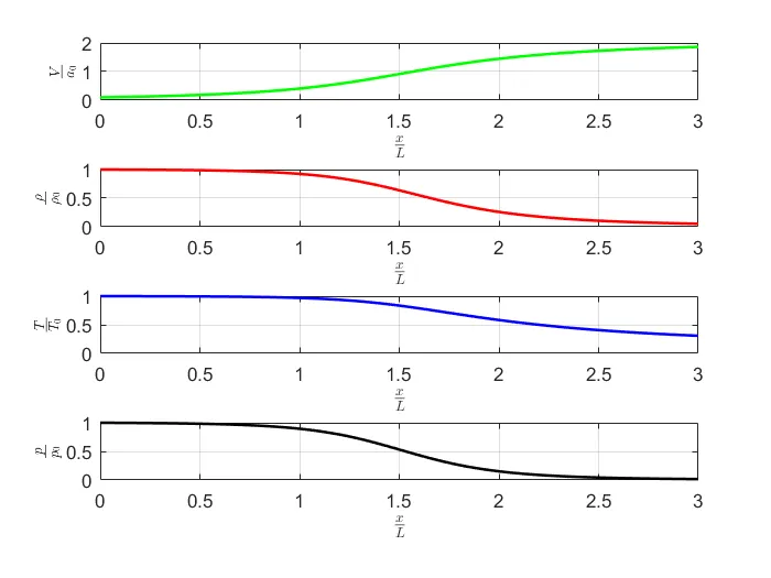
It can be seen that the velocity of the fluid increases at the end of the nozzle and the pressure drops along with the temperature and density.
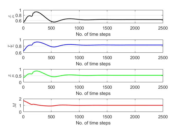
The transient variation of the primitive variables by solving the non-conservative form at the throat of the nozzle is shown below:
The variation of mass flow rate distribution inside the nozzle at different time steps during the time-marching process for the solution of the non-conservative form is shown below:
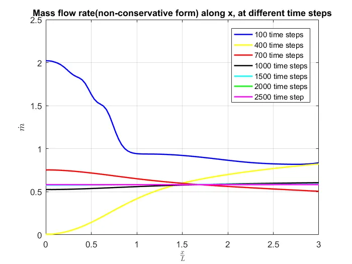
From the above figure, it can be seen that there is no much variation in mass flowrate after 1500 time steps. The same can be inferred from the image showing the transient variation of primitive variables also.
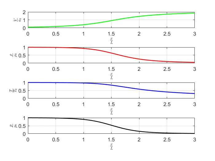
The steady-state distribution of the primitive variables by solving the conservative form of the governing equation is given below:
The transient variation of the primitive variables by solving the conservative form at the throat of the nozzle is shown below:
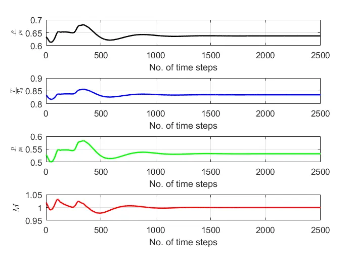
The variation of mass flow rate at different time steps for the conservative form of the governing equation is shown below:
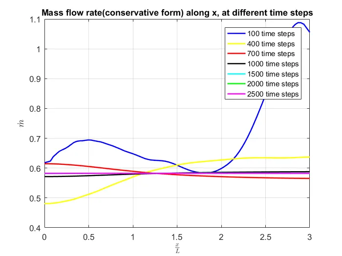
From the above figure, it can be seen that the flow becomes steady after 1500 timesteps.
By analyzing the above outputs it can be seen that there is no much difference in the final output even if the formulation is very different in the conservative and the non-conservative form. It is seen that the non-conservative form is easier to implement than the conservative form.
The comparison of the results obtained from the conservative and the non-conservative form can be done using the mass flow parameter in both the cases.
The plot showing the mass flow rate in both the cases, i.e the conservative and the non-conservative form is shown below:
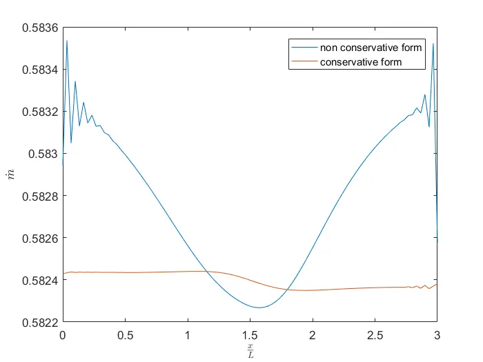
This is a highly zoomed view of the mass flow rate along the axis of the nozzle for the conservative and the non-conservative form. It is interesting to note that there are variations seen in the non-conservative form which are quite large but in the conservative form it is not very prominent. The analytical value of the mass flow parameter is 0.579 and the conservative form is much closer to the theoretical predictions. The zoomed-out view of the same image is given below:
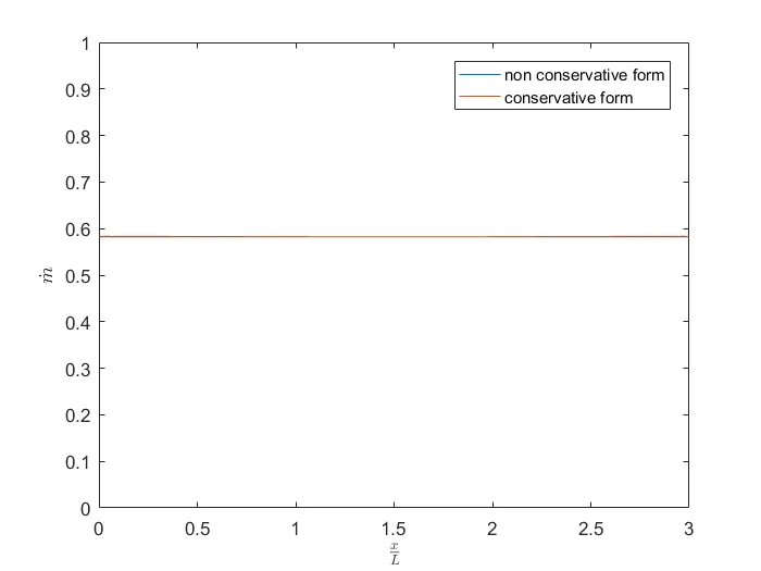
From the above figure, it can be seen that there are no large variations in the values computed using both the methods. So the numerical model we developed using Maccormack's method can be used in engineering calculations.
CONCLUSION
The simulation of the supersonic flow through a convergent-divergent nozzle is carried out using the Maccormack's method. The conservative and the non-conservative form of the governing equations are solved.
It is found that the simulation using the non-conservative form is easier to code and the time of execution is also small for the non-conservative form.
The conservative form tends to be more accurate, but there is no large difference in the computed solution in both cases.
APPENDIX
The codes used in post-processing is shown below:
clear all
close all
clc
% inputs


n= 91;
L = 3
x= linspace(0,L,n);
dx = L/(n-1);
throat = ((n-1)/2)+1;%calculate initial values
gamma = 1.4;
C =0.5;
% time steps
nt= 2500;
a = 1+2.2*(x-1.5).^2; % a = area


solver =2 % solver =1 non-conservative, solver = 2 conservative.
grid_time = linspace(0,nt,nt);
if solver ==1
% Initial conditions for the non-conservative form

 rho = 1-0.3146*x;
 T = 1-0.2314*x; % T= temperature
 v = (0.1+1.09*x).*T.^0.5;

 dt = min(C.*(dx./((T.^0.5)+v)));


 tic
% function for non-conservative form

 [rho,T,v,m,mach,dx,pr,rho_t,T_t,v_t,m_t,mach_t,pr_t] = non_conservative(x,n,nt,throat,rho,T,v,a,gamma,dt,dx)

 non_conservative_simulation_time = toc


elseif solver == 2
    for i = 1:n
    if (x(i)>=0 && x(i)<=0.5)
    rho2(i) = 1;
    T2(i) = 1;
    % T= temperature
    elseif (x(i)>=0.5 && x(i)<=1.5)
        rho2(i) = 1-0.366*(x(i)-0.5);
        T2(i) = 1-0.167*(x(i)-0.5);
    elseif (x(i)>=1.5 && x(i)<=3.5)
        rho2(i) = 0.634-0.3879*(x(i)-1.5);
        T2(i) = 0.833-0.3507*(x(i)-1.5);
    end
    end
    v2 = 0.59./(rho2.*a);

    dt = min(0.5.*(dx./((T2.^0.5)+v2)));


    tic
    [rho,T,v,m,mach,pr,rho_t,T_t,v_t,m_t,mach_t,pr_t] = conservative(x,n,nt,throat,rho2,T2,v2,a,gamma,dt,dx)
    cons_time = toc
end

% Post Processing

figure(2)
subplot(4,1,1)
plot(x,v,'color','g','linewidth',1.5)
xlabel('$\frac{x}{L}$','Interpreter','latex')
ylabel('$\frac{V}{a_0}$','Interpreter','latex')
grid()

subplot(4,1,2)
plot(x,rho,'color','r','linewidth',1.5)
xlabel('$\frac{x}{L}$','Interpreter','latex')
ylabel('$\frac{\rho}{\rho_0}$','Interpreter','latex')
grid()

subplot(4,1,3)
plot(x,T,'color','b','linewidth',1.5)
xlabel('$\frac{x}{L}$','Interpreter','latex')
ylabel('$\frac{T}{T_0}$','Interpreter','latex')
grid()


subplot(4,1,4)
plot(x,pr,'color','k','linewidth',1.5)
xlabel('$\frac{x}{L}$','Interpreter','latex')
ylabel('$\frac{p}{p_0}$','Interpreter','latex')
grid()


figure(3)
subplot(4,1,1)
plot(grid_time,rho_t,'color','k','linewidth',1.5)
xlabel('No. of time steps')
ylabel('$\frac{\rho}{\rho_0}$','Interpreter','latex')
grid()


subplot(4,1,2)
plot(grid_time,T_t,'color','b','linewidth',1.5)
xlabel('No. of time steps')
ylabel('$\frac{T}{T_0}$','Interpreter','latex')
grid()


subplot(4,1,3)
plot(grid_time,pr_t,'color','g','linewidth',1.5)
xlabel('No. of time steps')
ylabel('$\frac{p}{p_0}$','Interpreter','latex')
grid()


subplot(4,1,4)
plot(grid_time,mach_t,'color','r','linewidth',1.5)
xlabel('No. of time steps')
ylabel('$M$','Interpreter','latex')
grid()
In the above code the function for solving the conservative and the non-conservative form of the governing equations are called separately and the plots are generated.
The code used for comparing the mass flow rate is given below:
clear all
close all
clc
% inputs


n= 91;
L = 3
x= linspace(0,L,n);
dx = L/(n-1);
throat = ((n-1)/2)+1;%calculate initial values
gamma = 1.4;
C =0.5;
% time steps
nt= 2500;
a = 1+2.2*(x-1.5).^2; % a = area


grid_time = linspace(0,nt,nt);
% Initial conditions for the non-conservative form

 rho = 1-0.3146*x;
 T = 1-0.2314*x; % T= temperature
 v = (0.1+1.09*x).*T.^0.5;

 dt = min(C.*(dx./((T.^0.5)+v)));


% function for non-conservative form

 [rho,T,v,m,mach,dx,pr,rho_t,T_t,v_t,m_t,mach_t,pr_t] = non_conservative(x,n,nt,throat,rho,T,v,a,gamma,dt,dx)


    for i = 1:n
    if (x(i)>=0 && x(i)<=0.5)
    rho2(i) = 1;
    T2(i) = 1;
    % T= temperature
    elseif (x(i)>=0.5 && x(i)<=1.5)
        rho2(i) = 1-0.366*(x(i)-0.5);
        T2(i) = 1-0.167*(x(i)-0.5);
    elseif (x(i)>=1.5 && x(i)<=3.5)
        rho2(i) = 0.634-0.3879*(x(i)-1.5);
        T2(i) = 0.833-0.3507*(x(i)-1.5);
    end
    end
    v2 = 0.59./(rho2.*a);

    dt2 = min(0.5.*(dx./((T2.^0.5)+v2)));


    [rho2,T2,v2,m2,mach2,pr2,rho_t2,T_t2,v_t2,m_t2,mach_t2,pr_t2] = conservative(x,n,nt,throat,rho2,T2,v2,a,gamma,dt2,dx)

mass = rho.*v.*a

mass2 = rho2.*v2.*a

% Post Processing

figure(2)
plot(x,mass)
hold on
plot(x,mass2)
xlabel('$\frac{x}{L}$','Interpreter','latex')
ylabel('$\dot m$','Interpreter','latex')
legend('non conservative form','conservative form')

figure(3)
plot(x,mass)
hold on
plot(x,mass2)
xlabel('$\frac{x}{L}$','Interpreter','latex')
ylabel('$\dot m$','Interpreter','latex')
axis([0 3 0 1])
legend('non conservative form','conservative form')
The mass flow rate is saved in different variables mass and mass2 for the conservative and non-conservative forms. The above variables are used to plot the comparison in both the cases.