Simulation of a 1D Supersonic nozzle flow using MacCormack Method
OBJECTIVE: SIMULATION OF 1-D SUPERSONIC NOZZLE FLOW USING MACCORMACK METHOD
This challenge concerns the simulation of the fluid flow inside a converging-diverging nozzle. It also involves the study of the variation in the characteristics of the fluid properties along the length of the flow.
Any fluid flow problem in fluid mechanics is always solved using the basic two governing equations: the continuity equation and the momentum equation. If there is heat transfer involved then we shall use the energy equation too. These governing equations can be further classified into two categories: non-conservative and conservative form of the governing equations. The non-conservative form basically solves the independent flow variable like the density, velocity and tempurature. The conservative form on the other hand solves flux variables like the mass flux, momentum flux or the energy flux. The approach to solving these two forms of governing equations, though fundamentally equivalent, are quite different.
1-D SUPERSONIC NOZZLE FLOW SIMULATION USING THE CONSERVATIVE FORM OF THE GOVERNING EQUATIONS
a) THEORY
The governing fluid flow equations for the nozzle are all derived from the parent equation that is known as the Reynolds Transport Theorum. A general form of the Reynolds Transport Theorum is shown in the image below.
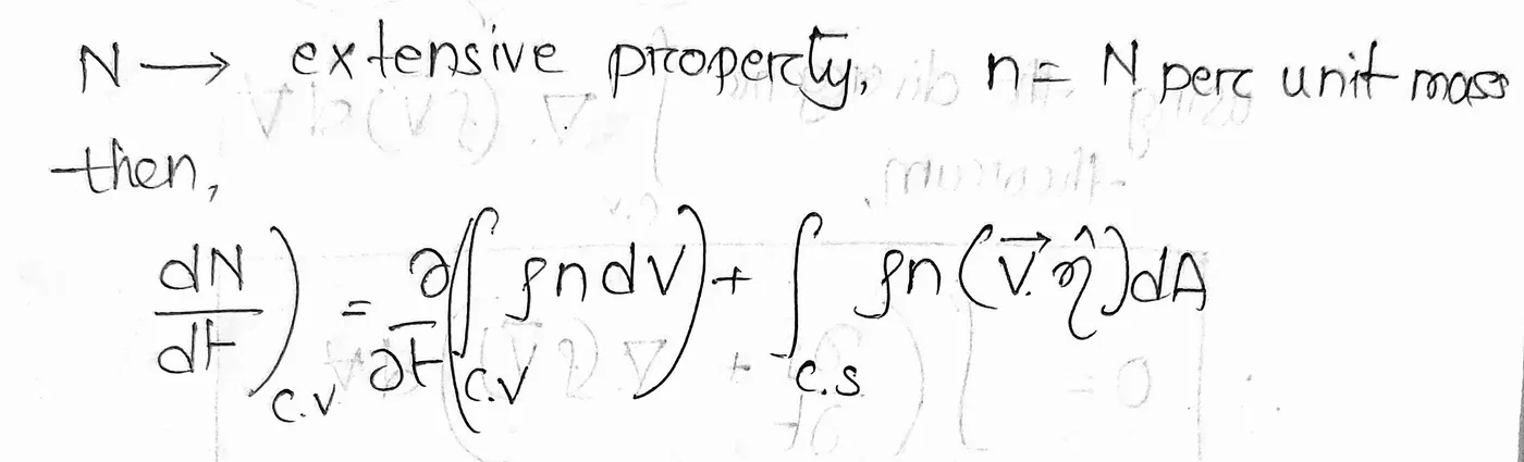
Here, 'N' refers to the property that we need to study in the control volume of the flow field and 'n' refers to that concerned property per unit mass. Based on this form of the Reynolds Transport Theorum, first the continuity equation was derived. The derivation is shown in the image shown below.
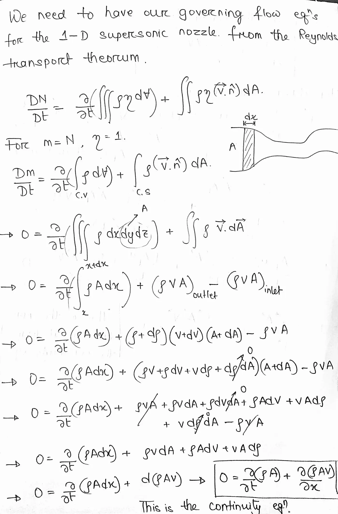
The equation derived above is the continuity equation in the dimensional form. When try to non-dimensionalize the variables in the equation, we obtain the non-dimensional form of the continuity equation. It is shown in the image below.
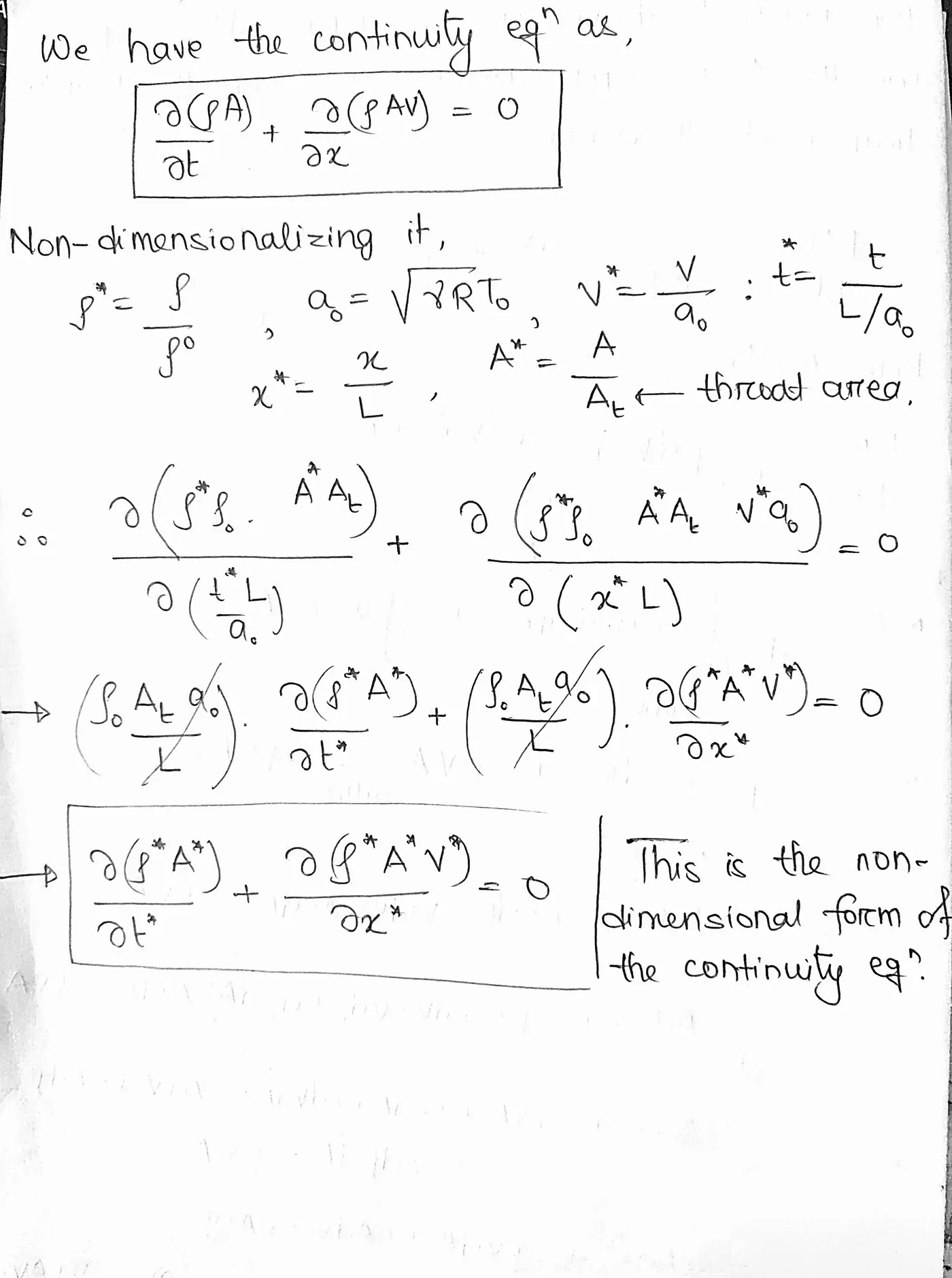
Now that we have both the dimensional and non-dimensional forms of our continuity equation, we shall derive our momentum equation from the Reynold's Transport Theorum too. The derivation is shown below in the image.
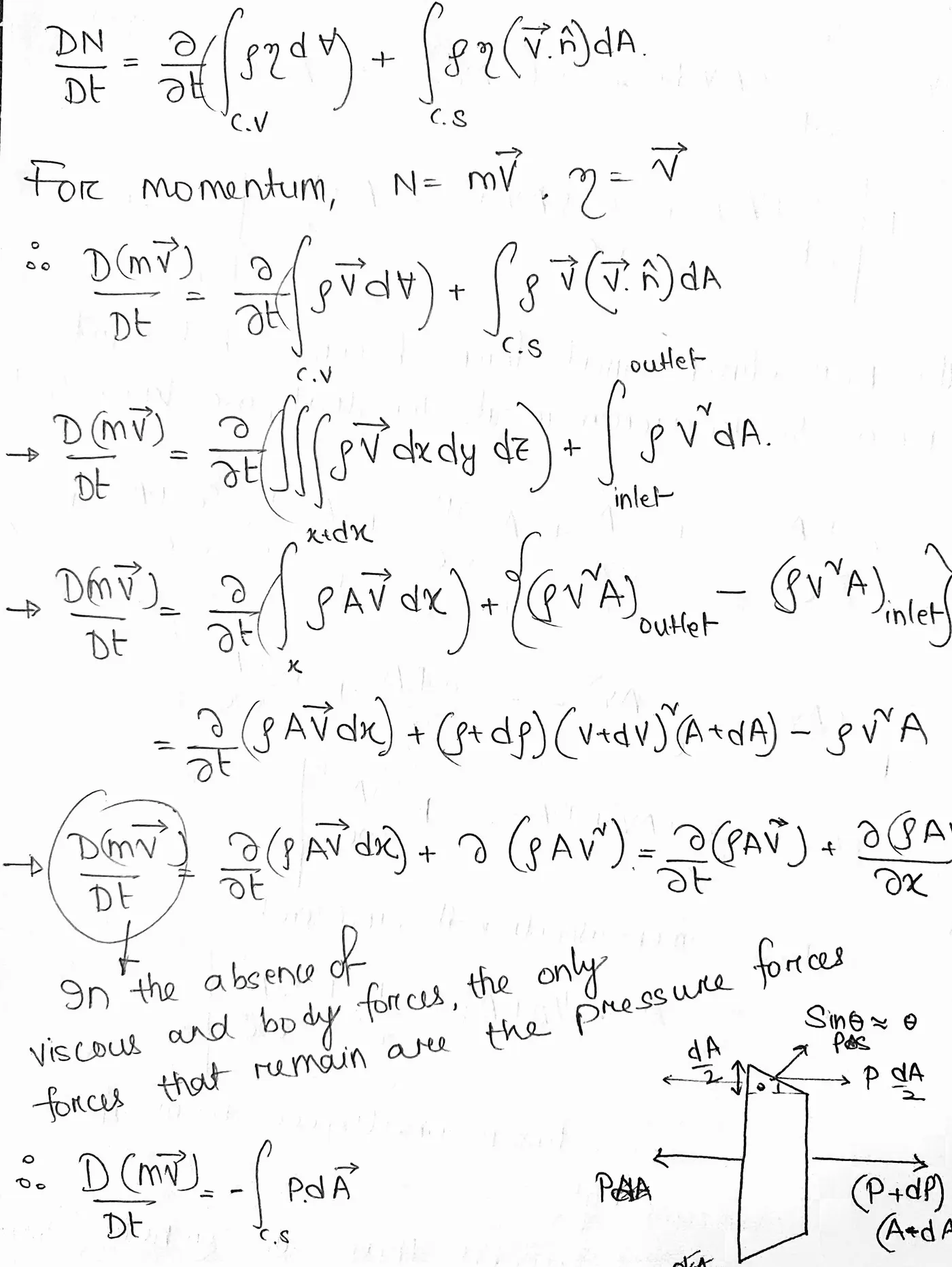
Fig.3(a):Derivation of Momentum Equation
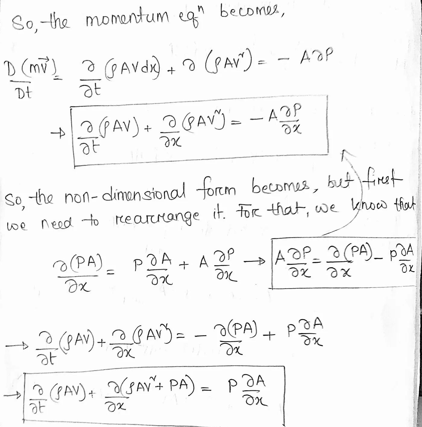
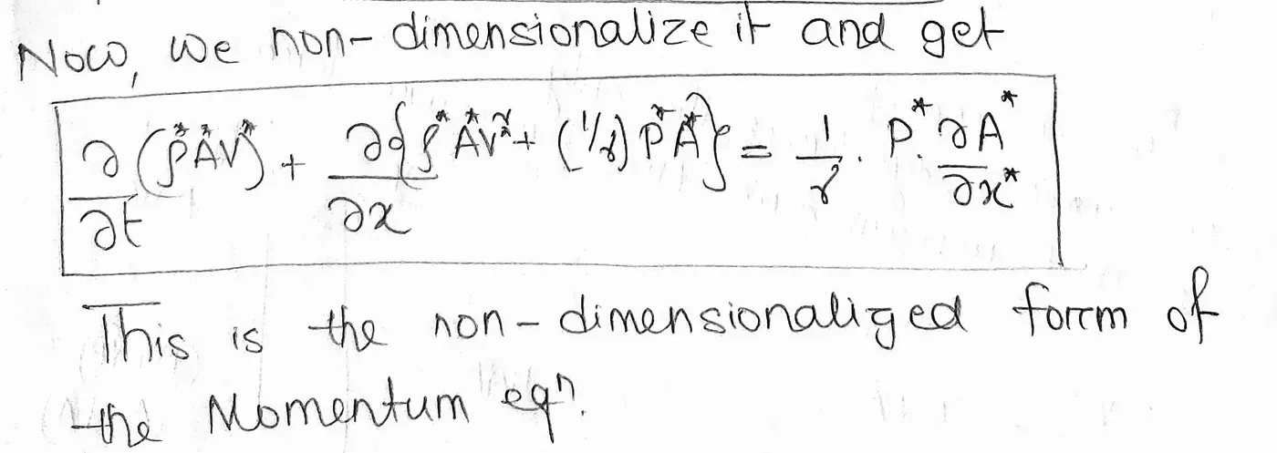
This form of the momentum equation is known as the dimensional form of the momentum equation. We now try to introduce the non-dimensional variables in the equation to convert this into the non-dimensional form of the momentum equation. It is shown below.
Similarly, using the Reynolds Transport Theorum and replacing 'N' with the Energy term, we arrive at the Energy equation. The equation is shown below in the image.
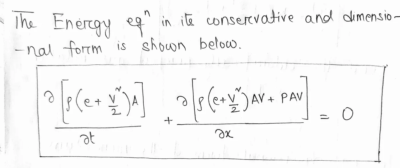
This is known as the dimensional form of the energy equation. We now try to convert this form into the non-dimensional form using the non-dimensional variables as shown in the image below.
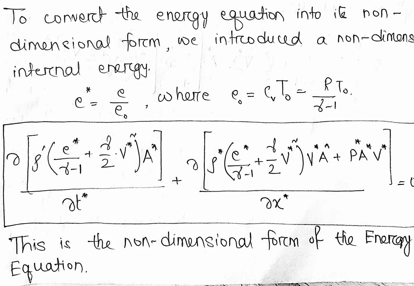
All the equations that have been derived from the Reynolds Transport Theorum above are known as the conservative form of the governing equations. The reason why these equations have been further reduced to their respective non-dimensional forms is primarily because most of the researchers in nozzle flows prefer to use non-dimensional variables for solving the equation as they feel it provides an aesthetic advantage while presenting the results (all the value remain between 0 and 1).
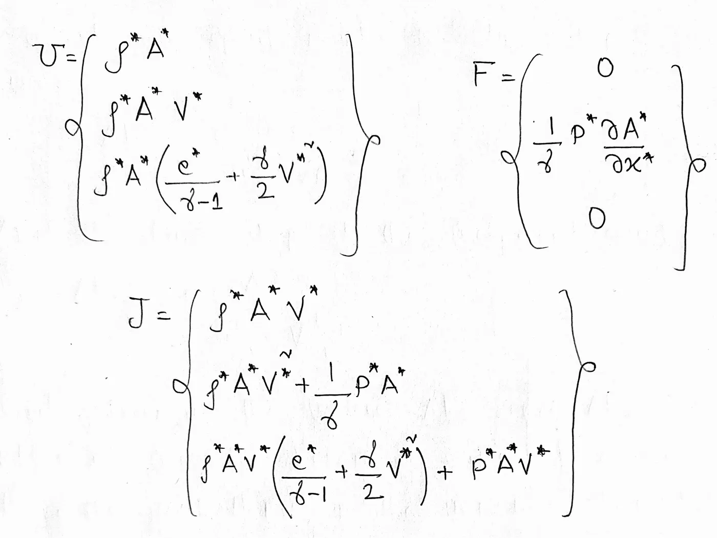
Now it has been observed that if we attempt to solve these equations numerically in terms of the primitive variables like the density and velocity(u,v,w), we do not obtain a solution. That is the reason we need to modify these equations further. The main advantage of using the conservative form is that the governing equations can be represented in a generic form. We attempt to group the time derivative, spatial derivative and the source term variables separately in the form of column vectors and name them U, J and F respectively. These vectors with its components are shown in the image below.
Hence, the governing differential equations that we had derived earlier now modifies to the following shown in the image below.
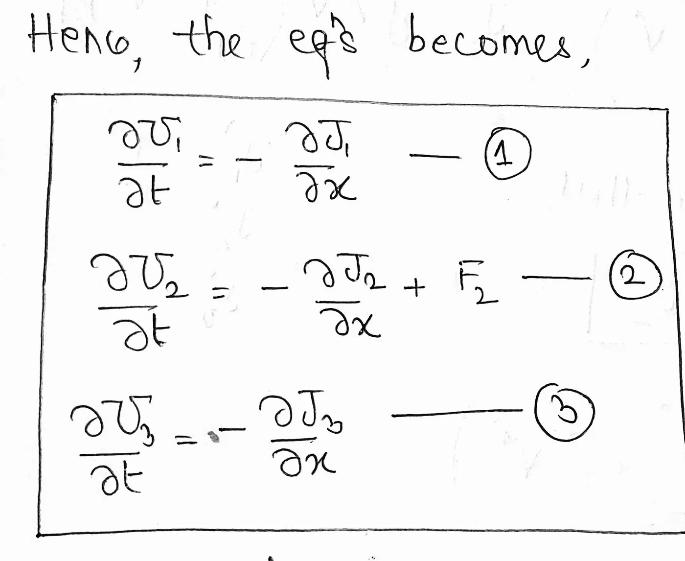
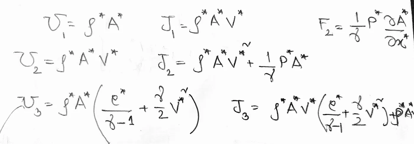
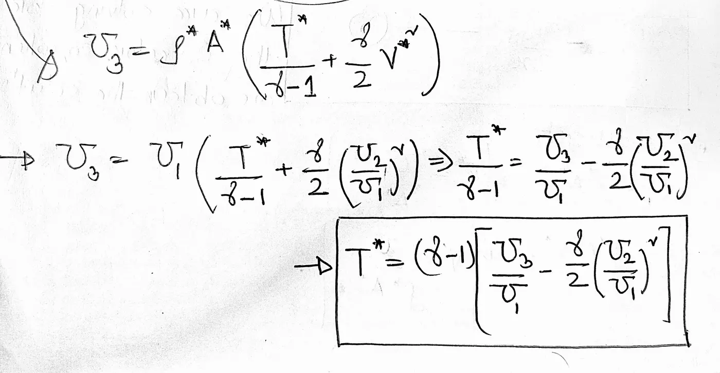
where equation (1), (2) & (3) are the continuity, momentum and the energy equations respectively. And their respective components are shown in the right hand side. We see here that U is the solution vector. So, to solve these equation and get the values of U1, U2 & U3, we shall express the J and F vectors in terms of the U vector. The transformation equations are shown in the image below.
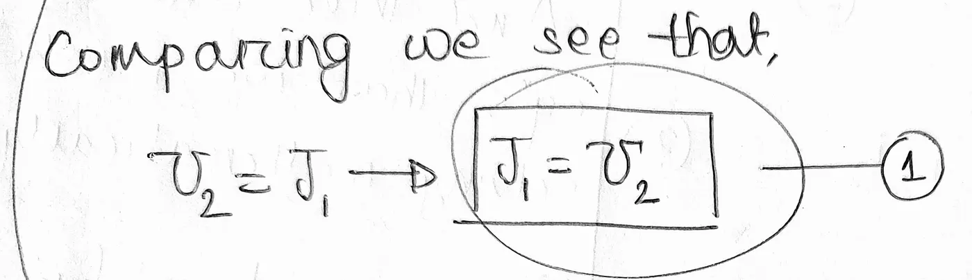
This is the equation expressing the J1 component in terms of the U2 component.
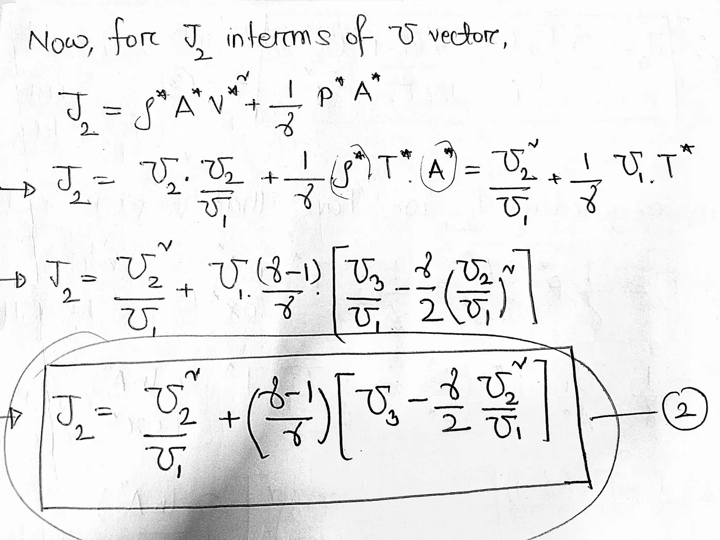
This concludes expressing the J2 component in terms of the U vector components.
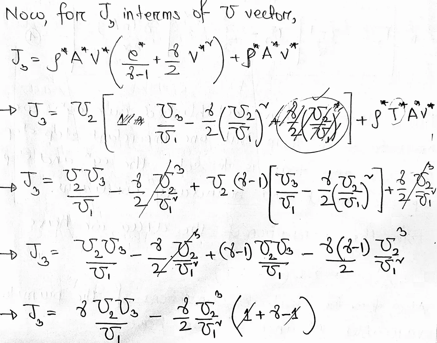

This is the expression for the J3 component interms of the U vector components.
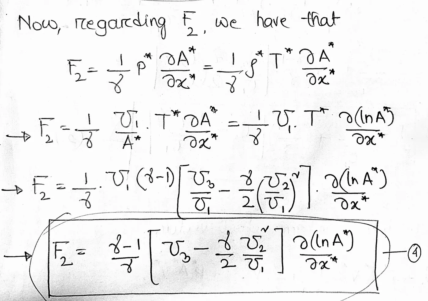
Now that we have obtained our transformed governing equation available to us, we can proceed to the next step of the solution which is the numerical discretization of these equations using the MacCormack Method.
b) Numerical Discretization
These non-dimensional form of the conservative equations will now be use to discretization using a very effective numerical technique known as the MacCormack Method.
The MacCormack method is an explicit finite-difference numerical technique that is used to discretize governing differential equations. It is based on a predictor-corrector method which means that the unknown variables are updated twice within a single time step.
a) Predictor Step: In this step, the spatial derivatives in the governing differentials equations are discretized using a forward difference scheme.
b) Corrector Step: In this step, the spatial derivatives in the governing differentials equations are discretized using a backward difference scheme.
c) Boundary Conditions
At the subsonic inflow boundary two properties are held fixed and one is allowed to float, and at the supersonic outflow boundary all properties are allowed to float. In the present formulation, we hold rho* and T* fixed at the inflow boundary, both equal to 1.0, and allow V* to float. By holding rho* fixed, then U1 at grid point i = 1 is fixed, independent of time, via U1 = rho*A*. That is,
U1 (i= 1) = (rho*A*) = A(i=1) = fixed value
The floating value of V' at the inflow boundary is calculated at the end of each time step by linearly extrapolating U2 from the known values at the internal grid points i = 2 and 3, that is,
U2(i=1) = 2U2(i=2) - U2(i=3)
Since V' floats at the inflow boundary, so does the value of U3 , which is given by
U3 = p*A*[(e*/(gamma-1)+(gamma/2)V*^2)]
As, U1 (i= 1) = (rho*A*) so the above equation becomes,
U3=U1[(e*/(gamma-1)+(gamma/2)V*^2)]
So, by putting the value of the tempurature, velocity and U1 flux, we shall be able to find the value of the U3 flux at the subsonic inlet of the nozzle. These values of the solution vector components U1, U2 and U3 at i=1 are then used to evalute the boundary values of the F and J vectors at the inlet. The flow properties at the downstream supersonic outflow boundary are obtained by linear extrapolation from the two adjacent internal points. If n denotes the grid point at the outflow boundary, then
U1(n) = 2U1(n-1) - U1(n-2)
U2(n) = 2U2(n-1) - U2(n-2)
U3(n) = 2U3(n-1) - U3(n-2)
Similar to the inlet, these values of the solution vector components U1, U2 and U3 at i=n are then used to evalute the boundary values of the F and J vectors at the supersonic outlet condition.
d) Initial Conditions
The nozzle that we shall assume in this case is a converging-diverging nozzle and hence its cross-sectional area does not remain constant. The profile for the nozzle walls is given by the following expression,
A(i)=1+2.2*(x(i)-1.5).^2
Since the dependent variables being solved using U1, U2, and U3 values, we shall need initial conditions for these variables at time t = 0 in order to start the finite-difference solution. The initial conditions for U1, U2, and U3 also allow for the calculation of the initial conditions of the F1, F2, F3 & J2 values. These independent variables (U vector) are further dependent of the values of the primitive variables of density, velocity and tempurature. Hence, it is essential to set the initial values of these primary variables to begin the finite difference approximations.
The initials conditions for the density, velocity and the tempurature are set such that two of these variables are determined and the third is allowed to float along the length of the nozzle. These intial conditions have been shown in the image below.
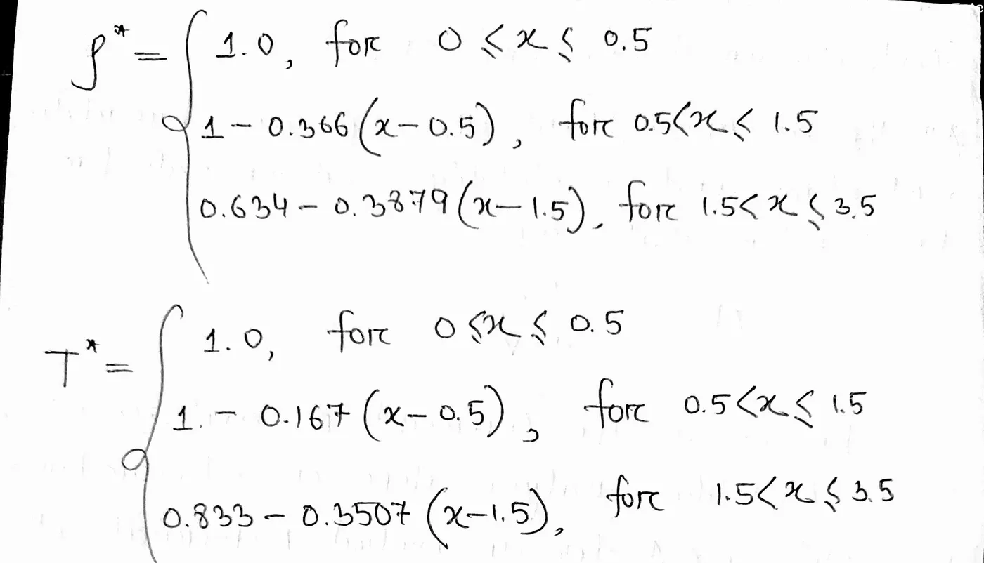
Here, Tempurature and density values have been initiated and the velocity is allowed to float. To calculate the value of the velocity at a particular node, we have
v(i)=U2(i)/U1(i)
where U2=rho*A*v, and is effectively the mass flow rate inside the nozzle at a particular node. So, to obtain the velocity at the inlet, we set an initial mass flow rate at the inlet of the nozzle which is U2(1)=0.59.
e) Calculation of the Time-Step
All the governing fluid flow equations are hyperbolic with respect to time and a stability condition exits for such a hyperbolic system that says,
dt=(C*dx)/(a+v)
C is known as the Courant number and according to the stability analysis done on a linear hyperbolic system of differential equations, C<=1 for a explicit numerical solution to be stable.
However, these equations in the current scenario are non-linear in nature, but even then this stability criterion C<=1 can be viewed as a general criterion for our non-linear system. In the stabilty condition, 'v' is the local velocity of the fluid flow at a point and 'a' is the local speed of sound. This stability condition along with C<=1 states that our time-step 'dt' should be atleast less than the time taken be a sound wave to travel from one grid point to another (dx). So, at any particular grid point the time-step is given by,
dt(i)=(C*dx)/(a(i)+v(i))
And the time-step at the adjacent grid shall be,
dt(i+1)=(C*dx)/(a(i+1)+v(i+1))
So, quite clearly we can see that time-steps at i and i+1 shall be different due to the differing values of the local fluid velocity 'v' and loccal sound speed 'a' along the grid. Hence, in the implementation of the time marching problem, we shall have two choices.
i) We can say that the values of the primitive variables for the next time-step can be found as,
rho(t+dt)=rho(t)+dt(t)*(drho/dt)(t)
In this manner, each of the flow variables shall proceed according to their own time-step. Hence, the resulting flow field at time 't+dt' will be in a type of artificial 'time wrap' with the flow field variables at a given grid point corresponding to some non-physical time different from that of the variables at an adjacent grid-point. Clearly, such a local time-stepping does not actually follow the real physical transients in the flow and hence does not produce an accurate solution.
However if the final steady state solution is the only thing that is desired then the local time stepping shall lead to faster convergence. But, the question remains whether this leads to the correct steady state.
ii) The other choice is to calculate the local time-step at each grid and then use the minimum value as the global time-step.
dt=min(dt(1),dt(2).........dt(n))
At this fashion, all the flow variables at all the grid points shall correspond to the same physical time. Hence, the time-marching solution is following the actual unsteady variations that exists in nature.
f) Code for the solution of the conservative form of the Governing Differential equations
clear all
close all
clc
tic
%length of the domain
L=3;

%No. of grid elements
n=31;

gamma=1.4;

%forming the mesh domain
x=linspace(0,L,n);
%grid size
dx=x(2)-x(1);

%variation of area of cross-section of the nozzle
A=1+2.2*(x-1.5).^2;

%Initial conditions for the primitive varibales in the nozzle


for i = 1:n
  %The two fixed variables that were fixed in the initial conditions was the density and tempurature variation.
  %The third variable 'velocity was allowed to float with the grid points.

   if (x(i)>=0 && x(i)<=0.5)
       rho(i)=1;
       T(i)=1;
   end

   if (x(i)>0.5 && x(i)<=1.5)
       rho(i)=1-0.366*(x(i)-0.5);
       T(i)=1-0.167*(x(i)-0.5);
   end

   if (x(i)>1.5 && x(i)<=3)
       rho(i)=0.634-0.3879*(x(i)-1.5);
       T(i)=0.833-0.3507*(x(i)-1.5);
   end

   %We find the floating variables of velocity using the mass flux variable U2 where U2=m_dot where m_dot is the mass flow rate in the nozzle.
   %so the Velocity becomes

   %v(i)=m_initial(i)/(rho(i).*A(i));

   m_initial(i)=0.59;    %Theoretical Mass Flow Rate ratio

   v(i)=m_initial(i)/(rho(i)*A(i));

end


%Initial conditions for the Derived flux variables of the nozzle

U1=rho.*A;                                               %Mass
U2=rho.*A.*v;                                            %Momentum
U3=rho.*((T/(gamma-1))+(gamma/2)*v.^2).*A;               %Energy

%Solving the governing equation using the MacCormack Method


for k=1:1400

  %The governing equations of Continuity, Momentum and Energy Equation has been expressed in term of the flux variables that have been derived as a function of the primitive varibales of rho, T and v
  %Continuity Equation:   dU1/dt+dF1/dx=0;
  %Momentum Equation:     dU2/dt+dF2/dx=J2;
  %Energy Equation:       dU3/dt+dF3/dx=0;

  %Saving the old Values
  U1_old=U1;
  U2_old=U2;
  U3_old=U3;

  F1=U2;
  F2=((U2.^2)./U1) + (((gamma-1)/gamma)*(U3 - ((gamma*0.5*(U2.^2))./U1)));
  F3=((gamma*U2.*U3)./U1) - ((gamma*0.5*(gamma-1)*(U2.^3))./(U1.^2));

  %PREDICTOR STEP

    for i=2:n-1

        J2(i)=(1/gamma)*rho(i)*T(i)*((A(i+1)-A(i))/dx);

        %Continuity Equation

        dU1_dt_p(i)=-(F1(i+1)-F1(i))/dx;

        %Momentum Equation

        dU2_dt_p(i)=-(F2(i+1)-F2(i))/dx+J2(i);

        %Energy Equation

        dU3_dt_p(i)=-(F3(i+1)-F3(i))/dx;

        %defining the time step
        %We know that the time step at any grid point is given by the
        %expression

        %dt(i)=(C*dx)/(a(i)=v(i));

        %where C is the courant number and a is the velocity of sound. For a
        %stable explicit scheme to yield converging results the courant number
        %should be C=<1.0

        C=0.5;
        %Also the non-dimensional expression for the Velocity of sound is given
        %as

        a=sqrt(T);
        dt=min((C*dx)./(a(i)+v(i)));


        %calculating the new values
        U1(i)=U1_old(i)+dt*dU1_dt_p(i);
        U2(i)=U2_old(i)+dt*dU2_dt_p(i);
        U3(i)=U3_old(i)+dt*dU3_dt_p(i);

        rho(i) = U1(i)/A(i);
        v(i) = U2(i)/U1(i);
        T(i) = (gamma-1)*((U3(i)/U1(i)) - ((gamma/2)*(v(i)^2)));

    end

    %CORRECTOR STEP

    F1=U2;
    F2=((U2.^2)./U1) + (((gamma-1)/gamma)*(U3 - ((gamma*0.5*(U2.^2))./U1)));
    F3=((gamma*U2.*U3)./U1) - ((gamma*0.5*(gamma-1)*(U2.^3))./(U1.^2));


    for i=2:n-1

        J2(i)=(1/gamma)*rho(i)*T(i)*((A(i)-A(i-1))/dx);

        %Continuity Equation

        dU1_dt_c(i)=-(F1(i)-F1(i-1))/dx;

        %Momentum Equation

        dU2_dt_c(i)=-(F2(i)-F2(i-1))/dx+J2(i);

        %Enenrgy Equation

        dU3_dt_c(i)=-(F3(i)-F3(i-1))/dx;


    end

    %Calculating the average of the change
    dU1_dt=0.5*(dU1_dt_p+dU1_dt_c);
    dU2_dt=0.5*(dU2_dt_p+dU2_dt_c);
    dU3_dt=0.5*(dU3_dt_p+dU3_dt_c);

    %Calculating the new values
    for i=2:n-1

        U1(i)=U1_old(i)+dt*dU1_dt(i);
        U2(i)=U2_old(i)+dt*dU2_dt(i);
        U3(i)=U3_old(i)+dt*dU3_dt(i);

        rho(i)= U1(i)/A(i);

    end

    %Density
    rho = U1./A;

    %Velocity
    v = U2./U1;

    %Tempurature
    T = (gamma-1)*((U3./U1) - ((gamma/2)*(v.^2)));

    % Boundary Nodes

    % Inlet
    U1(1) = rho(1)*A(1);
    U2(1) = 2*U2(2) - U2(3);
    U3(1) = U1(1)*((T(1)/(gamma-1))+(0.5*gamma*(v(1)^2)));

    %Outlet
    U1(n) = 2*U1(n-1) - U1(n-2);
    U2(n) = 2*U2(n-1) - U2(n-2);
    U3(n) = 2*U3(n-1) - U3(n-2);

    %Mach no.
    a=sqrt(T);   %speed of sound
    M=v./a;

    %Mass Flow Rate inside the nozzle
    m=rho.*A.*v;

    %Fluid Properties at the throat
    rho_t(k)=rho(16);
    v_t(k)=v(16);
    T_t(k)=T(16);

    figure(6)
            hold on
            if k==50
                plot(x,m,'g','linewidth',1);
            else if k==100
                plot(x,m,'k','linewidth',1);
                else if k==150
                    plot(x,m,'b','linewidth',1);
                    else if k==200
                        plot(x,m,'y','linewidth',1);
                        else if k==700
                            plot(x,m,'r','linewidth',1)
                                else if k==1400
                                    plot(x,m,'m','linewidth',1)
                                    legend('50dt','100dt','150dt','200dt','700dt','1400dt');
                                    title('Mass flow rate in a nozzle wrt time step for conservative form');
                                    xlabel('nozzle length(x/L)')
                                    ylabel('mass flow rate(rho*v*A/rho_0*v_0*A_0)')
                                    end
                            end
                        end
                    end
                end
            end
    figure(1)
    plot(x,v,'red')
    xlabel('Nozzle length(x/L)')
    ylabel('Fluid velocity(v/v_0)')
    legend('Velocity')

    title(sprintf('Time-Step:%d',k));

    figure(2)
    plot(x,rho,'blue')
    xlabel('Nozzle length(x/L)')
    ylabel('Fluid Density(rho/rho_0)')
    legend('density')

    title(sprintf('Time-Step:%d',k));

    figure(3)
    plot(x,T,'green')
    xlabel('Nozzle length(x/L)')
    ylabel('Fluid Tempurature(T/T_0)')
    legend('Tempurature')

    title(sprintf('Time-Step:%d',k));

    figure(4)
    plot(x,M,'yellow')
    xlabel('Nozzle length')
    ylabel('Fluid Mach Number')
    legend('Mach Number')

    title(sprintf('Time-Step:%d',k));

    figure(5)
    plot(x,m,'black')
    ylim([0.580 0.6]);
    xlabel('Nozzle length(x/L)')
    ylabel('Nozzle Mass Flow rate(rho*v*A/rho_0*v_0*A_0)')
    legend('Mass Flow Rate')

    title(sprintf('Time-Step:%d',k));

    pause(0.01)
    hold off

end

subplot(311)
plot(1:k,rho_t)
ylabel('Density rho/rho_0')
xlabel('No. of time-steps')
title('Timewise Variation of Density at the throat');

subplot(312)
plot(1:k,v_t)
ylabel('Velocity v/v_0')
xlabel('No. of time-steps')
title('Timewise Variation of Velocity at the throat');

subplot(313)
plot(1:k,T_t)
ylabel('Temperature T/T_0')
xlabel('No. of time-steps')
title('Timewise Variation of Temperature at the throat');
g) Results
i) Velocity
ii) Density
iii) Tempurature
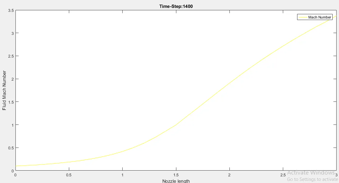
iv) Mach Number
v) Mass Flow Rate
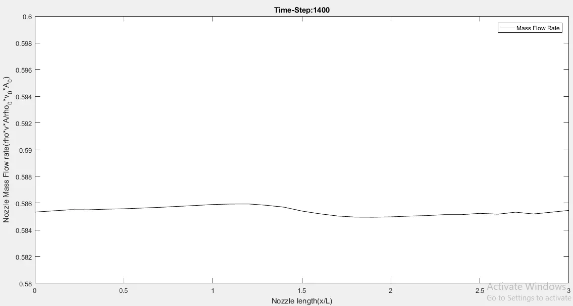
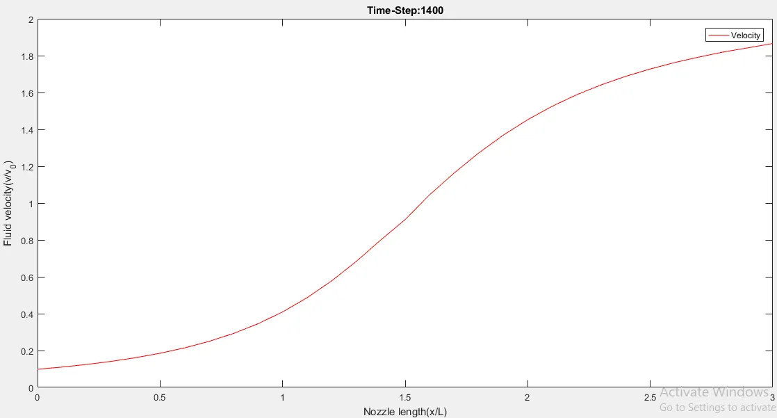
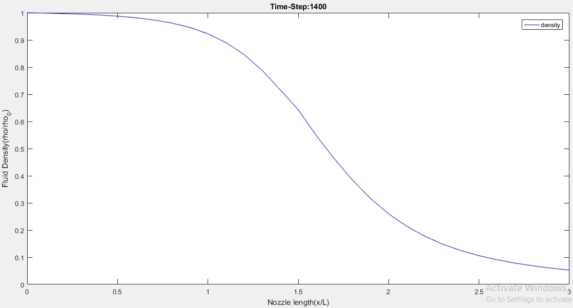
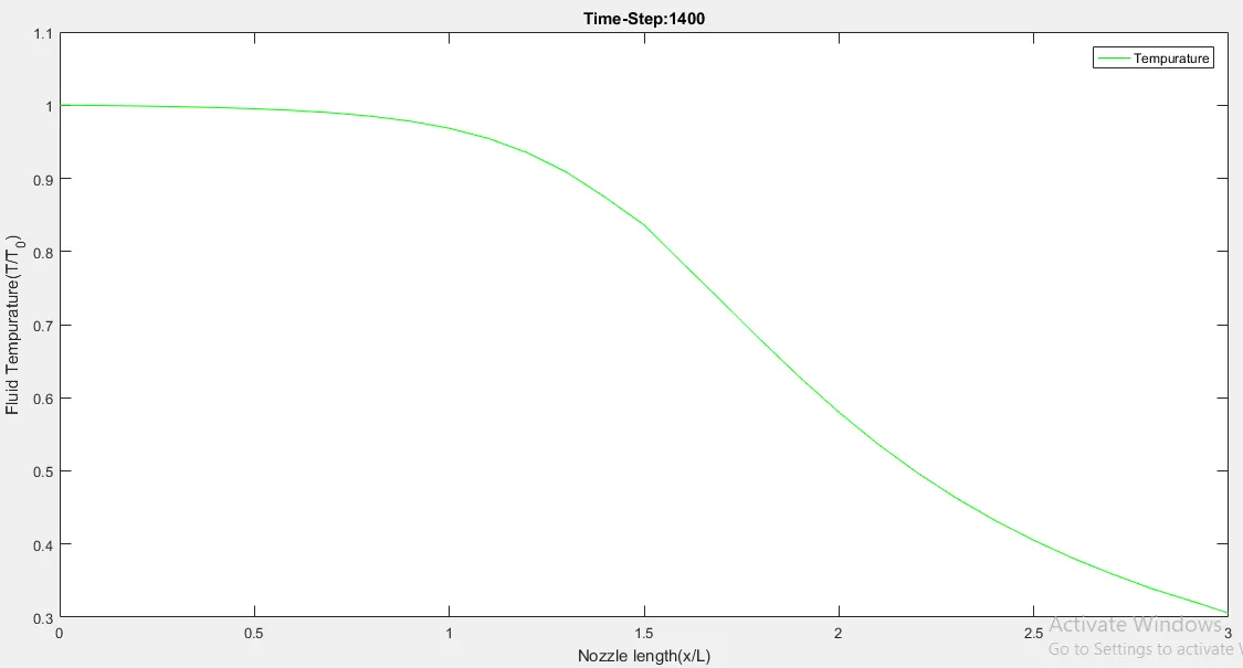
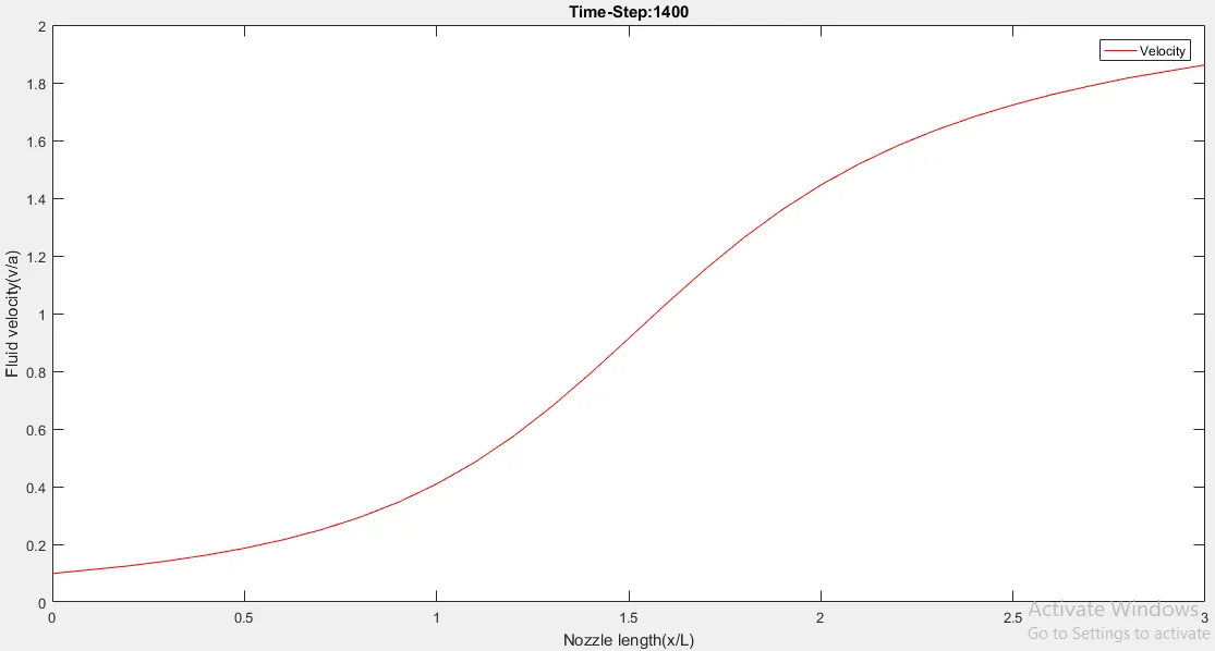
The above plots are the results that show up when we try to solve the 1-D supersonic nozzle flow problem using the conservative form of the governing equations. The variations of the non-dimensional fluid properties have been plotted against the non-dimensional nozzle length.
Also the comparison for the mass flow rate inside the nozzle for different time-steps i.e how the solution for the mass flow rate develops inside the nozzle with time is shown in the graph below.
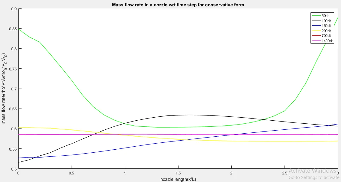
In this graph we see that, as we march ahead in time, the mass flow rate distribution becomes more and more steady along the length of the nozzle. At around 700-1400 time steps, the mass flow rate distribution becomes nearly horizantal indicating that it has reached a steady state value which is close to actual analytical mass flow rate of 0.59.
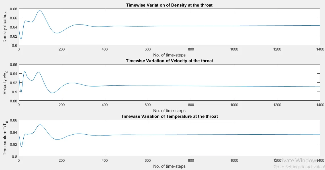
The study of timewise variation of the fluid flow properties was also carried out with the nozzle throat as the reference. It showed that the density, velocity and the tempurature values reached steady state value beyond 400 timesteps. The plots are shown below.
1-D SUPERSONIC NOZZLE FLOW SIMULATION USING THE NON-CONSERVATIVE FORM OF THE GOVERNING EQUATIONS
a) THEORY
In the previous case, we have seen that all the governing fluid flow equations are derived using the Reynolds Transport Theorum. The equations, thus obtained, were refered to as the conservative form of the governing equations. These equations solved the flux variables inside the nozzle such as the mass flux, momentum flux and the energy flux and from these variable we were able to extract the variations of the values of the primitive variables along the length of the nozzle.
Now, we shall move over to the solution of the 1-D Supersonic Flow inside the nozzle using the non-conservative form of the governing equations. First, the continuity equation used for this analysis is given as,
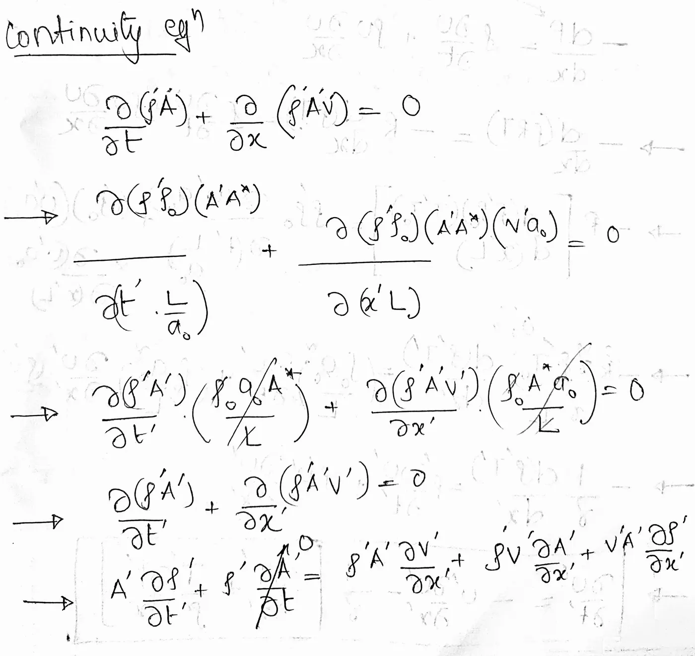
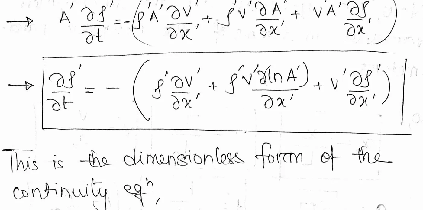
We observe that the derivation again starts from the conservative form of the continuity equation. The variables in these expressions are all in their non-dimensional form. The main difference that we can see in these expression compared to the conservative form is that here the equation is solved directly for the primitive variables.
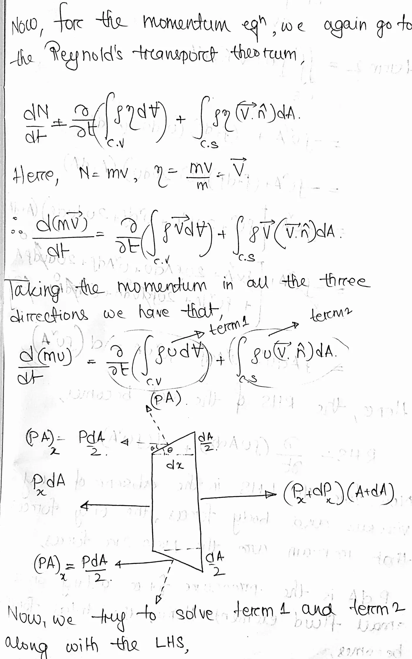
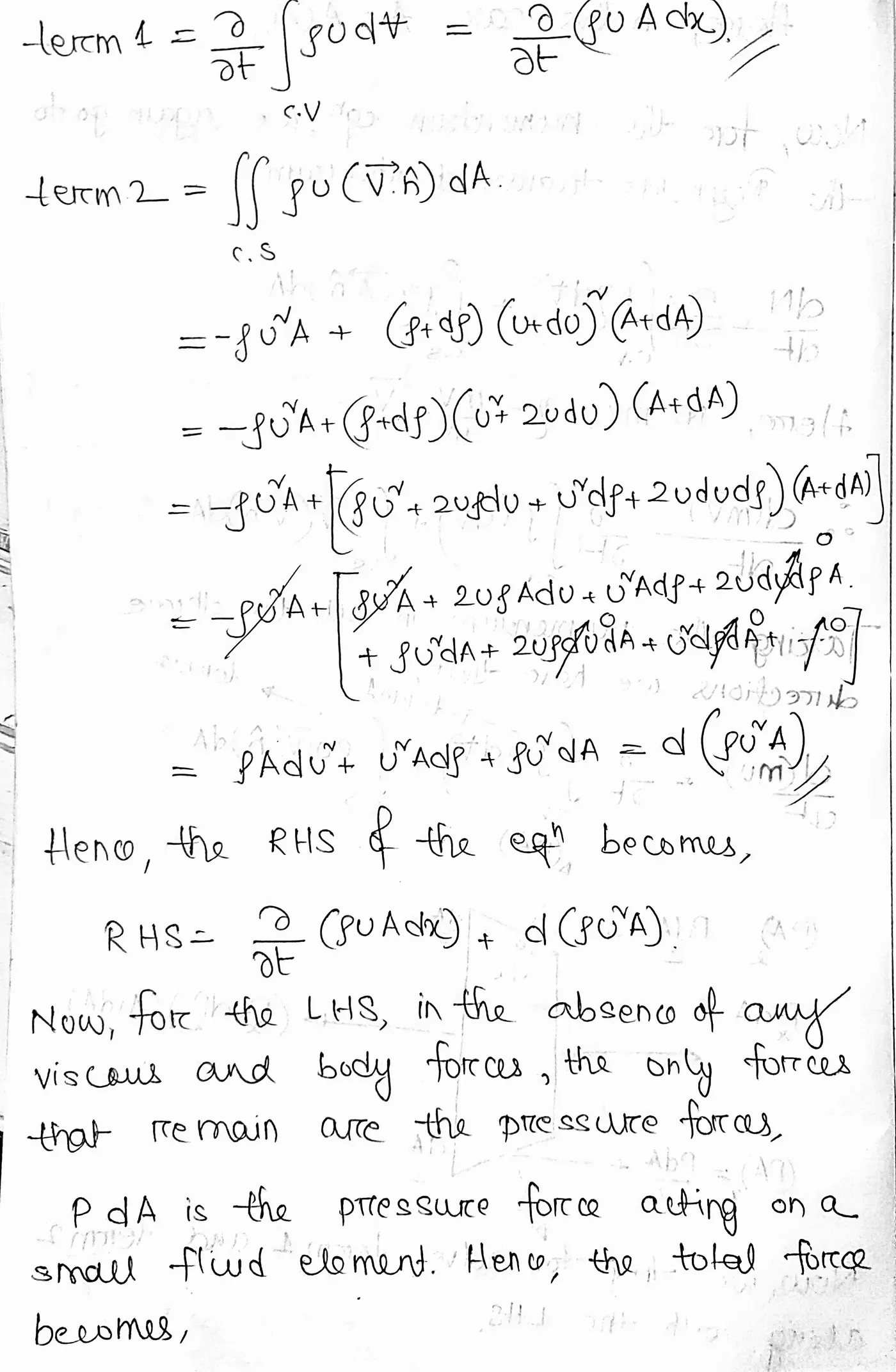
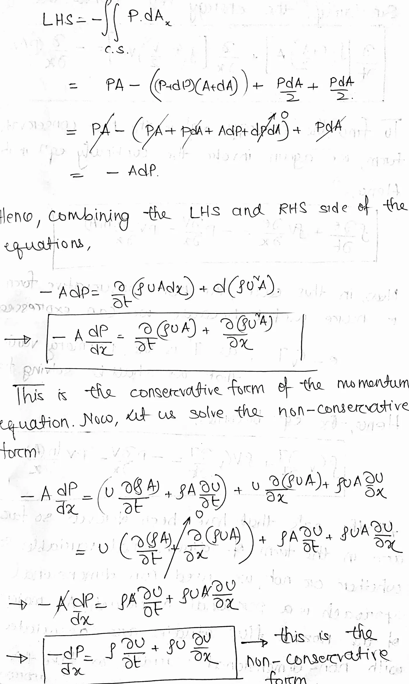
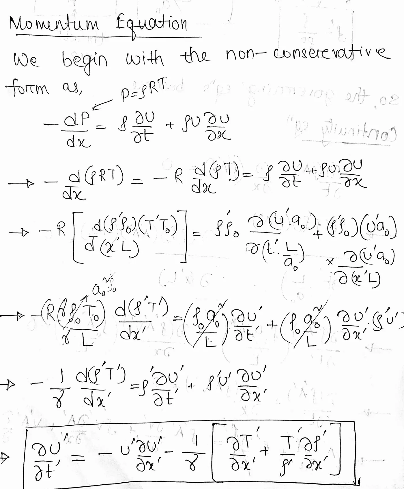
The expression above represents the non-conservative form of the momentum equation in its non-dimensional form. Its derivation starts again from the Reynolds Trnasport Theorum as in case of its conservative counterpart.
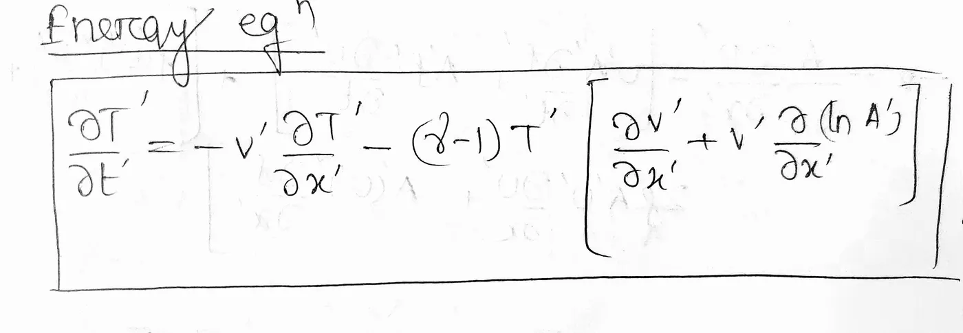
The expression above represents the non-conservative form of the Energy equation in its non-dimensional form.
Now that we have obtained our governing equation available to us, we can proceed to the next step of the solution which is the numerical discretization of these equations using the MacCormack Method.
b) Numerical Discretization
These non-dimensional form of the conservative equations will now be use to discretization using a very effective numerical technique known as the MacCormack Method.
The MacCormack method is an explicit finite-difference numerical technique that is used to discretize governing differential equations. It is based on a predictor-corrector method which means that the unknown variables are updated twice within a single time step.
a) Predictor Step: In this step, the spatial derivatives in the governing differentials equations are discretized using a forward difference scheme.
b) Corrector Step: In this step, the spatial derivatives in the governing differentials equations are discretized using a backward difference scheme.
c) Boundary Conditions
Subsonic inflow boundary (point 1): We allow one variable to float. We choose the velocity v1, because on a physical basis we know the mass flow through the nozzle must be allowed to adjust to the proper steady state, and allowing v1 to float makes the most sense as part of this adjustment. The value of v1 changes with time and is calculated from information provided by the flow-field solution over the internal points, (The internal points are those not on a boundary, i.e, points 2 through n-1). We use linear extrapolation from points 2 and 3 to
calculate v1. The slope of the linear extrapolation line is determined from points 2 and 3 as
Slope= [v(2) - v(3)]/dx
Using this slope to find v1 by linear extrapolation, we have
v(1)=v(2)-slope=v(2)-[v(2)-v(3)]/dx
v(1) = 2v(2) - v(3)
All other flow-field variables are specified. Since point 1 is viewed as essentially the reservoir, we stipulate the density and temperature at point 1 to be their respective stagnation values, Po and To, respectively. These are held.fixed, independent of time. Hence, in terms of the non-dimensional variables, we have
T(1)=1
rho(1)=1
Supersonic outflow boundary (point N): Here, we must allow all flow-field variables to float. We again choose to use linear extrapolation based on the flowfield values at the internal points. Specifically, we have, for the nondimensional variables,
v(n) = 2v(n-1) - v(n-2)
rho(n) = 2rho(n-1) - rho(n-2)
T(n)= 2T(n-1) - T(n-1)
d) Nozzle Shape and Initial Conditions
The nozzle that we shall assume in this case is a converging-diverging nozzle and hence its cross-sectional area does not remain constant along the length. The profile for the nozzle walls is given by the following expression,
A(i)=1+2.2*(x(i)-1.5).^2
The initials conditions for the density, velocity and the tempurature are set such that two of these variables are determined and the third is allowed to float along the length of the nozzle. These intial conditions have been shown in the image below.
Here, Tempurature and density values have been initiated and the velocity is allowed to float. To calculate the value of the velocity at a particular node, we have
v(i)=U2(i)/U1(i)
where U2=rho*A*v, and is effectively the mass flow rate inside the nozzle at a particular node. So, to obtain the velocity at the inlet, we set an initial mass flow rate at the inlet of the nozzle which is U2(1)=0.59.
e) Calculation of the Time-Step
All the governing fluid flow equations are hyperbolic with respect to time and a stability condition exits for such a hyperbolic system that says,
dt=(C*dx)/(a+v)
C is known as the Courant number and according to the stability analysis done on a linear hyperbolic system of differential equations, C<=1 for a explicit numerical solution to be stable.
However, these equations in the current scenario are non-linear in nature, but even then this stability criterion C<=1 can be viewed as a general criterion for our non-linear system. In the stabilty condition, 'v' is the local velocity of the fluid flow at a point and 'a' is the local speed of sound. This stability condition along with C<=1 states that our time-step 'dt' should be atleast less than the time taken be a sound wave to travel from one grid point to another (dx). So, at any particular grid point the time-step is given by,
dt(i)=(C*dx)/(a(i)+v(i))
And the time-step at the adjacent grid shall be,
dt(i+1)=(C*dx)/(a(i+1)+v(i+1))
So, quite clearly we can see that time-steps at i and i+1 shall be different due to the differing values of the local fluid velocity 'v' and loccal sound speed 'a' along the grid. Hence, in the implementation of the time marching problem, we shall have two choices.
i) We can say that the values of the primitive variables for the next time-step can be found as,
rho(t+dt)=rho(t)+dt(t)*(drho/dt)(t)
In this manner, each of the flow variables shall proceed according to their own time-step. Hence, the resulting flow field at time 't+dt' will be in a type of artificial 'time wrap' with the flow field variables at a given grid point corresponding to some non-physical time different from that of the variables at an adjacent grid-point. Clearly, such a local time-stepping does not actually follow the real physical transients in the flow and hence does not produce an accurate solution.
However if the final steady state solution is the only thing that is desired then the local time stepping shall lead to faster convergence. But, the question remains whether this leads to the correct steady state.
ii) The other choice is to calculate the local time-step at each grid and then use the minimum value as the global time-step.
dt=min(dt(1),dt(2).........dt(n))
At this fashion, all the flow variables at all the grid points shall correspond to the same physical time. Hence, the time-marching solution is following the actual unsteady variations that exists in nature.
f) Code for the solution of the non-conservative form of the Governing Differential equations
clear all
close all
clc

%length of the domain
L=3;

%No. of grid elements
n=31;

gamma=1.4;

%forming the mesh domain
x=linspace(0,L,n);
%grid size
dx=x(2)-x(1);

%Calculating the initial conditions
rho=1-0.3146*x;                  %Density
T=1-0.2314*x;                    %Tempurature
v=(0.1+1.09*x).*T.^0.5;          %Velocity
A=1+2.2*(x-1.5).^2;              %Area

%Theoretical Mass Flow Rate
for i=1:n
   m_initial(i)=rho(i)*A(i)*v(i);
end

%solving for the 1-D supersonic flow through the nozzle using
%non-conservative equations,

%time loop
for k=1:1400

    rho_old=rho;
    v_old=v;
    T_old=T;

    %predictor step

    for i=2:n-1

    %defining the time step
    %We know that the time step at any grid point is given by the
    %expression

    %dt(i)=(C*dx)/(a(i)=v(i));

    %where C is the courant number and a is the velocity of sound. For a
    %stable explicit scheme to yield converging results the courant number
    %should be C=<1.0

    C=0.5;

    %Also the non-dimensional expression for the Velocity of sound is given
    %as
    a=sqrt(T);
    dt=min((C*dx)./(a(i)+v(i)));
    %This shall be the time-step for each and every grid of the nozzle
    %domain which means that each and every grid element of the nozzle
    %shall be solved using a unique time-step.


    dv_dx=(v(i+1)-v(i))/dx;
    dlogA_dx=(log(A(i+1))-log(A(i)))/dx;
    drho_dx=(rho(i+1)-rho(i))/dx;
    dT_dx=(T(i+1)-T(i))/dx;

    %continuity equation
    drho_dt_p(i)=-rho(i)*dv_dx-rho(i)*v(i)*dlogA_dx-v(i)*drho_dx;

    %momentum equation
    dv_dt_p(i)=-v(i)*dv_dx-(1/gamma)*(dT_dx+(T(i)/rho(i))*drho_dx);

    %Energy Equation
    dT_dt_p(i)=-v(i)*dT_dx-(gamma-1)*T(i)*(dv_dx+v(i)*dlogA_dx);

    %updating the values for the predictor step
    rho(i)=rho(i)+drho_dt_p(i)*dt;         %density
    v(i)=v(i)+dv_dt_p(i)*dt;               %velocity
    T(i)=T(i)+dT_dt_p(i)*dt;

    end


    %corrector method

    %defining the time step again using the updated value of the flow
    %variables
    a=sqrt(T);
    dt=min((C*dx)./(a+v));

    for i=2:n-1

    dv_dx=(v(i)-v(i-1))/dx;
    dlogA_dx=(log(A(i))-log(A(i-1)))/dx;
    drho_dx=(rho(i)-rho(i-1))/dx;
    dT_dx=(T(i)-T(i-1))/dx;

    %continuity equation
    drho_dt_c(i)=-rho(i)*dv_dx-rho(i)*v(i)*dlogA_dx-v(i)*drho_dx;

    %momentum equation
    dv_dt_c(i)=-v(i)*dv_dx-(1/gamma)*(dT_dx+(T(i)/rho(i))*drho_dx);

    %Energy Equation
    dT_dt_c(i)=-v(i)*dT_dx-(gamma-1)*T(i)*(dv_dx+v(i)*dlogA_dx);


    end

    %computing the Average derivative
    drho_dt=0.5*(drho_dt_p+drho_dt_c);
    dv_dt=0.5*(dv_dt_p+dv_dt_c);
    dT_dt=0.5*(dT_dt_p+dT_dt_c);

    %Computing the values
    for i=2:n-1
        rho(i)=rho_old(i)+drho_dt(i)*dt;
        v(i)=v_old(i)+dv_dt(i)*dt;
        T(i)=T_old(i)+dT_dt(i)*dt;
    end

    % Boundary conditions at Inlet
    v(1) = 2*v(2)-v(3);
    rho(1) = 1;
    T(1) = 1;
    % Boundary conditions at outlet
    v(n) = 2*v(n-1) - v(n-2);
    rho(n)=2*rho(n-1) - rho(n-2);
    T(n) = 2*T(n-1) - T(n-2);

    %Calculating the Mach no. of the flow along the nozzle
    a=sqrt(T);

    M=v./a;

    %Calculating the Mass Flowrate along the nozzle length
    m=rho.*A.*v;

    rho_t(k)=rho(16);
    v_t(k)=v(16);
    T_t(k)=T(16);

    figure(6)
    if k==50
        plot(x,m,'g','linewidth',1)
        hold on
    else if k==100
            plot(x,m,'y','linewidth',1)
            hold on
        else if k==200
                plot(x,m,'b','linewidth',1)
                hold on
            else if k==500
                    plot(x,m,'r','linewidth',1)
                    hold on
                else if k==700
                        plot(x,m,'black','linewidth',1)
                        hold on

                        legend('50dt','100dt','200dt','500dt','700dt')
                        xlabel('nozzle length(x/L)')
                        ylabel('mass flow rate(rho*v*A/rho_0*v_0*A_0)')

                        title('Mass flow rate in a nozzle wrt time step for non-conservative form');
                    end
                end
            end
        end
    end

    figure(1)
    plot(x,v,'red')
    xlabel('Nozzle length(x/L)')
    ylabel('Fluid velocity(v/a)')
    legend('Velocity')

    title(sprintf('Time-Step:%d',k));

    figure(2)
    plot(x,rho,'blue')
    xlabel('Nozzle length(x/L)')
    ylabel('Fluid Density(rho/rho_0)')
    legend('density')


    title(sprintf('Time-Step:%d',k));

    figure(3)
    plot(x,T,'green')
    xlabel('Nozzle length(x/L)')
    ylabel('Fluid Tempurature(T/T_o)')
    legend('Tempurature')

    title(sprintf('Time-Step:%d',k));

    figure(4)
    plot(x,M,'yellow')
    xlabel('Nozzle length(x/L)')
    ylabel('Fluid Mach Number(M)')
    legend('Mach Number')

    title(sprintf('Time-Step:%d',k));

    figure(5)
    plot(x,m_initial,'--')
    hold on
    plot(x,m,'black')
    xlabel('Nozzle length')
    ylabel('Nozzle Mass Flow rate')
    legend('Mass Flow Rate')
    ylim([0.58 0.60])
    title(sprintf('Time-Step:%d',k));

    pause(0.001)
    hold off

end
subplot(311)
plot(1:k,rho_t)
ylabel('Density rho/rho_0')
xlabel('No. of time-steps')
title('Timewise Variation of Density at the throat');

subplot(312)
plot(1:k,v_t)
ylabel('Velocity v/v_0')
xlabel('No. of time-steps')
title('Timewise Variation of Velocity at the throat');

subplot(313)
plot(1:k,T_t)
ylabel('Temperature T/T_0')
xlabel('No. of time-steps')
title('Timewise Variation of Temperature at the throat');
g) Results
i) Velocity
ii) Density
iii) Tempurature
iv) Mach Number
v) Mass Flow rate
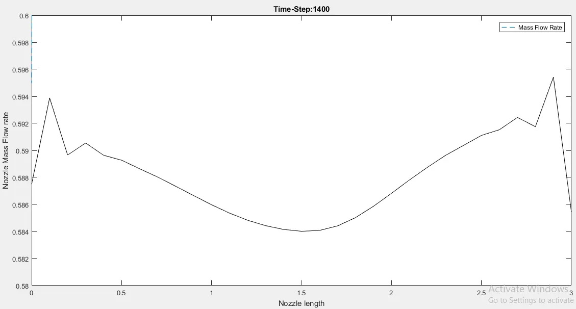
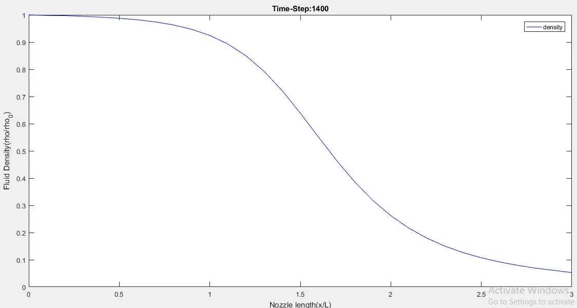
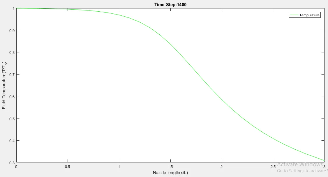
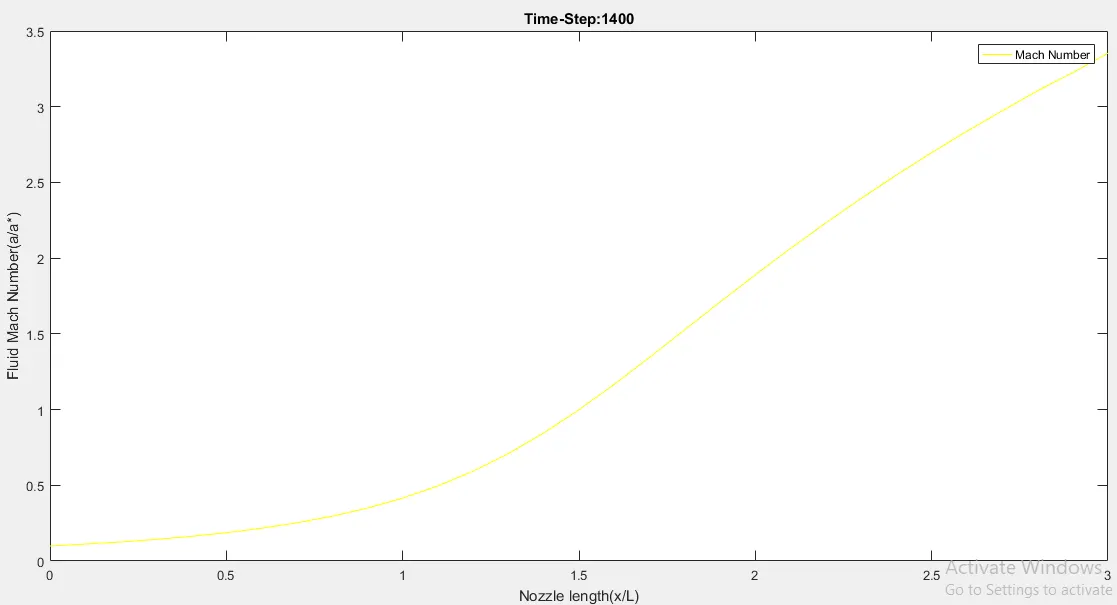
The above plots are the results that show up when we try to solve the 1-D supersonic nozzle flow problem using the conservative form of the governing equations. The variations of the non-dimensional fluid properties have been plotted against the non-dimensional nozzle length.
Also the comparison for the mass flow rate inside the nozzle for different time-steps i.e how the solution for the mass flow rate develops inside the nozzle with time is shown in the graph below.
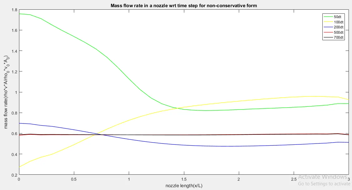
In this graph we see that, as we march ahead in time, the mass flow rate distribution becomes more and more steady along the length of the nozzle. At around 700 time steps, the mass flow rate distribution becomes nearly horizantal indicating that it has reached a steady state value which is close to actual analytical mass flow rate of 0.59.
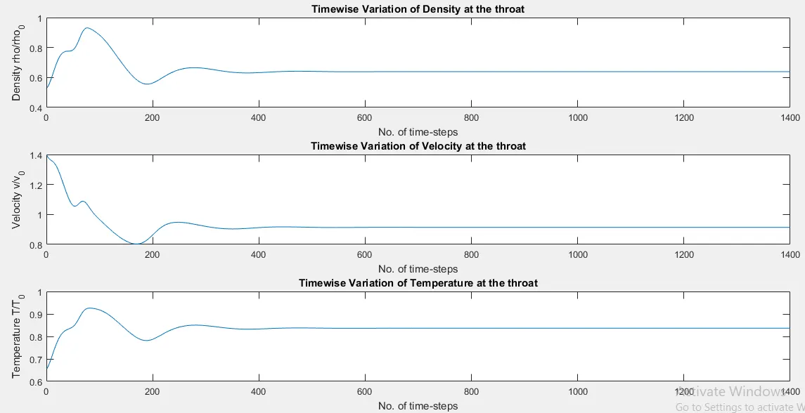
The study of timewise variation of the fluid flow properties was also carried out with the nozzle throat as the reference. It showed that the density, velocity and the tempurature values reached steady state value beyond 400 timesteps. The plots are shown below.
CONSERVATIVE VS NON-CONSERVATIVE FORM OF THE GOVERNING EQUATIONS
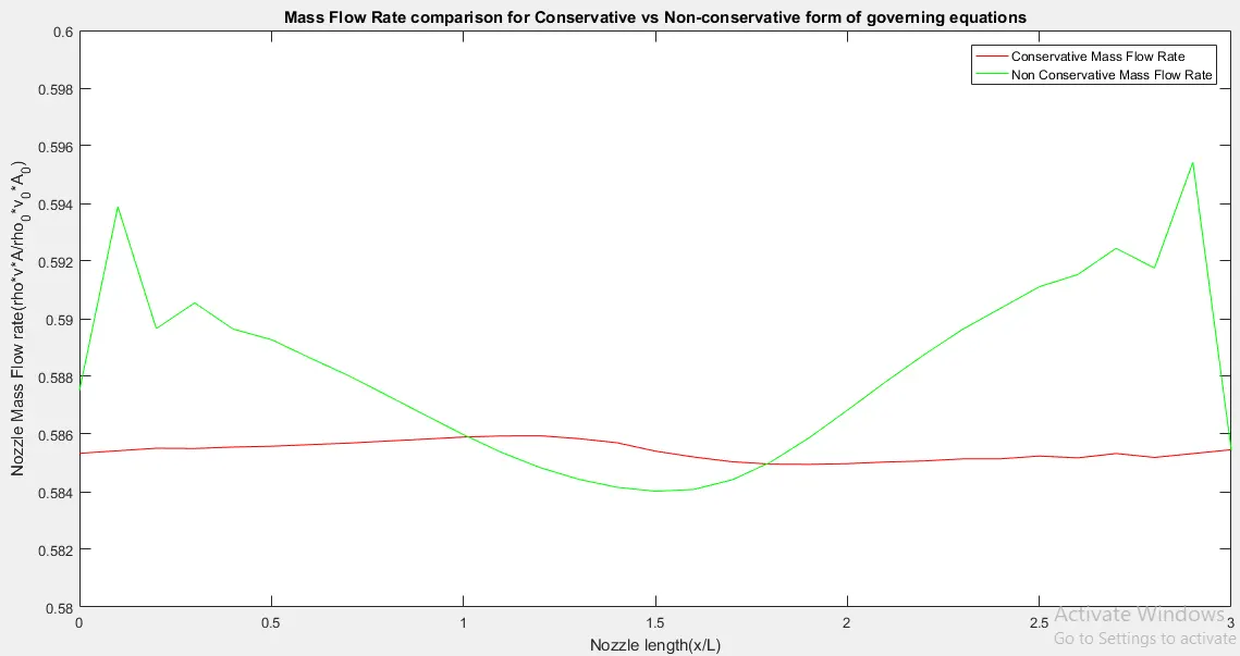
To compare the accuracy of the results obtained using both the conservative as well as the non-conservative form of the governing equations, another code was written to compare the variation in the mass flow rate inside the nozzle under steady state. This code is shown below.
clear all
close all
clc

%length of the domain
L=3;

%No. of grid elements
n=31;

gamma=1.4;

%forming the mesh domain
x=linspace(0,L,n);
%grid size
dx=x(2)-x(1);

%variation of area of cross-section of the nozzle
A=1+2.2*(x-1.5).^2;

%Initial conditions for the primitive varibales in the nozzle


for i = 1:n
  %The two fixed variables that were fixed in the initial conditions was the density and tempurature variation.
  %The third variable 'velocity was allowed to float with the grid points.

   if (x(i)>=0 && x(i)<=0.5)
       rho_initial(i)=1;
       T_initial(i)=1;
   end

   if (x(i)>0.5 && x(i)<=1.5)
       rho_initial(i)=1-0.366*(x(i)-0.5);
       T_initial(i)=1-0.167*(x(i)-0.5);
   end

   if (x(i)>1.5 && x(i)<=3)
       rho_initial(i)=0.634-0.3879*(x(i)-1.5);
       T_initial(i)=0.833-0.3507*(x(i)-1.5);
   end

   %We find the floating variables of velocity using the mass flux variable U2 where U2=m_dot where m_dot is the mass flow rate in the nozzle.
   %so the Velocity becomes

   %v(i)=m_initial(i)/(rho(i).*A(i));

   m_initial(i)=0.59;    %Theoretical Mass Flow Rate ratio

   v_initial(i)=m_initial(i)/(rho_initial(i)*A(i));

end

rho_actual=rho_initial;
v_actual=v_initial;
T_actual=T_initial;
%Initial conditions for the Derived flux variables of the nozzle

U1=rho_actual.*A;                                                       %Mass
U2=rho_actual.*A.*v_initial;                                            %Momentum
U3=rho_actual.*((T_actual/(gamma-1))+(gamma/2)*v_actual.^2).*A;       %Energy

%Solving the governing equation using the MacCormack Method

%time loop for conservative form
for k=1:1400

  %The governing equations of Continuity, Momentum and Energy Equation has been expressed in term of the flux variables that have been derived as a function of the primitive varibales of rho, T and v
  %Continuity Equation:   dU1/dt+dF1/dx=0;
  %Momentum Equation:     dU2/dt+dF2/dx=J2;
  %Energy Equation:       dU3/dt+dF3/dx=0;

  %Saving the old Values
  U1_old=U1;
  U2_old=U2;
  U3_old=U3;

  F1=U2;
  F2=((U2.^2)./U1) + (((gamma-1)/gamma)*(U3 - ((gamma*0.5*(U2.^2))./U1)));
  F3=((gamma*U2.*U3)./U1) - ((gamma*0.5*(gamma-1)*(U2.^3))./(U1.^2));

  %PREDICTOR STEP

    for i=2:n-1

        J2(i)=(1/gamma)*rho_actual(i)*T_actual(i)*((A(i+1)-A(i))/dx);

        %Continuity Equation

        dU1_dt_p(i)=-(F1(i+1)-F1(i))/dx;

        %Momentum Equation

        dU2_dt_p(i)=-(F2(i+1)-F2(i))/dx+J2(i);

        %Energy Equation

        dU3_dt_p(i)=-(F3(i+1)-F3(i))/dx;

        %defining the time step
        %We know that the time step at any grid point is given by the
        %expression

        %dt(i)=(C*dx)/(a(i)=v(i));

        %where C is the courant number and a is the velocity of sound. For a
        %stable explicit scheme to yield converging results the courant number
        %should be C=<1.0

        C=0.5;
        %Also the non-dimensional expression for the Velocity of sound is given
        %as

        a=sqrt(T_actual);
        dt=min((C*dx)./(a(i)+v_actual(i)));


        %calculating the new values
        U1(i)=U1_old(i)+dt*dU1_dt_p(i);
        U2(i)=U2_old(i)+dt*dU2_dt_p(i);
        U3(i)=U3_old(i)+dt*dU3_dt_p(i);

        rho_actual(i) = U1(i)/A(i);
        v_actual(i) = U2(i)/U1(i);
        T_actual(i) = (gamma-1)*((U3(i)/U1(i)) - ((gamma/2)*(v_actual(i)^2)));

    end

    %CORRECTOR STEP

    F1=U2;
    F2=((U2.^2)./U1) + (((gamma-1)/gamma)*(U3 - ((gamma*0.5*(U2.^2))./U1)));
    F3=((gamma*U2.*U3)./U1) - ((gamma*0.5*(gamma-1)*(U2.^3))./(U1.^2));


    for i=2:n-1

        J2(i)=(1/gamma)*rho_actual(i)*T_actual(i)*((A(i)-A(i-1))/dx);

        %Continuity Equation

        dU1_dt_c(i)=-(F1(i)-F1(i-1))/dx;

        %Momentum Equation

        dU2_dt_c(i)=-(F2(i)-F2(i-1))/dx+J2(i);

        %Enenrgy Equation

        dU3_dt_c(i)=-(F3(i)-F3(i-1))/dx;


    end

    %Calculating the average of the change
    dU1_dt=0.5*(dU1_dt_p+dU1_dt_c);
    dU2_dt=0.5*(dU2_dt_p+dU2_dt_c);
    dU3_dt=0.5*(dU3_dt_p+dU3_dt_c);

    %Calculating the new values
    for i=2:n-1

        U1(i)=U1_old(i)+dt*dU1_dt(i);
        U2(i)=U2_old(i)+dt*dU2_dt(i);
        U3(i)=U3_old(i)+dt*dU3_dt(i);

    end

    %Density
    rho_actual = U1./A;

    %Velocity
    v_actual = U2./U1;

    %Tempurature
    T_actual = (gamma-1)*((U3./U1) - ((gamma/2)*(v_actual.^2)));

    % Boundary Nodes

    % Inlet
    U1(1) = rho_actual(1)*A(1);
    U2(1) = 2*U2(2) - U2(3);
    U3(1) = U1(1)*((T_actual(1)/(gamma-1))+(0.5*gamma*(v_actual(1)^2)));

    %Outlet
    U1(n) = 2*U1(n-1) - U1(n-2);
    U2(n) = 2*U2(n-1) - U2(n-2);
    U3(n) = 2*U3(n-1) - U3(n-2);

    %Mach no.
    a=sqrt(T_actual);   %speed of sound
    M=v_actual./a;

    %Mass Flow Rate inside the nozzle
    m_conservative=rho_actual.*A.*v_actual;


end


%time loop for non-conservative form
for k=1:1400

    rho_old=rho_initial;
    v_old=v_initial;
    T_old=T_initial;

    %predictor step

    for i=2:n-1

    %defining the time step
    %We know that the time step at any grid point is given by the
    %expression

    %dt(i)=(C*dx)/(a(i)=v(i));

    %where C is the courant number and a is the velocity of sound. For a
    %stable explicit scheme to yield converging results the courant number
    %should be C=<1.0

    C=0.5;

    %Also the non-dimensional expression for the Velocity of sound is given
    %as
    a=sqrt(T_initial);
    dt=min((C*dx)./(a(i)+v_initial(i)));
    %This shall be the time-step for each and every grid of the nozzle
    %domain which means that each and every grid element of the nozzle
    %shall be solved using a unique time-step.


    dv_dx=(v_initial(i+1)-v_initial(i))/dx;
    dlogA_dx=(log(A(i+1))-log(A(i)))/dx;
    drho_dx=(rho_initial(i+1)-rho_initial(i))/dx;
    dT_dx=(T_initial(i+1)-T_initial(i))/dx;

    %continuity equation
    drho_dt_p(i)=-rho_initial(i)*dv_dx-rho_initial(i)*v_initial(i)*dlogA_dx-v_initial(i)*drho_dx;

    %momentum equation
    dv_dt_p(i)=-v_initial(i)*dv_dx-(1/gamma)*(dT_dx+(T_initial(i)/rho_initial(i))*drho_dx);

    %Energy Equation
    dT_dt_p(i)=-v_initial(i)*dT_dx-(gamma-1)*T_initial(i)*(dv_dx+v_initial(i)*dlogA_dx);

    %updating the values for the predictor step
    rho_initial(i)=rho_initial(i)+drho_dt_p(i)*dt;         %density
    v_initial(i)=v_initial(i)+dv_dt_p(i)*dt;               %velocity
    T_initial(i)=T_initial(i)+dT_dt_p(i)*dt;

    end


    %corrector method

    %defining the time step again using the updated value of the flow
    %variables
    a=sqrt(T_initial);
    dt=min((C*dx)./(a+v_initial));

    for i=2:n-1

    dv_dx=(v_initial(i)-v_initial(i-1))/dx;
    dlogA_dx=(log(A(i))-log(A(i-1)))/dx;
    drho_dx=(rho_initial(i)-rho_initial(i-1))/dx;
    dT_dx=(T_initial(i)-T_initial(i-1))/dx;

    %continuity equation
    drho_dt_c(i)=-rho_initial(i)*dv_dx-rho_initial(i)*v_initial(i)*dlogA_dx-v_initial(i)*drho_dx;

    %momentum equation
    dv_dt_c(i)=-v_initial(i)*dv_dx-(1/gamma)*(dT_dx+(T_initial(i)/rho_initial(i))*drho_dx);

    %Energy Equation
    dT_dt_c(i)=-v_initial(i)*dT_dx-(gamma-1)*T_initial(i)*(dv_dx+v_initial(i)*dlogA_dx);


    end

    %computing the Average derivative
    drho_dt=0.5*(drho_dt_p+drho_dt_c);
    dv_dt=0.5*(dv_dt_p+dv_dt_c);
    dT_dt=0.5*(dT_dt_p+dT_dt_c);

    %Computing the values
    for i=2:n-1
        rho_initial(i)=rho_old(i)+drho_dt(i)*dt;
        v_initial(i)=v_old(i)+dv_dt(i)*dt;
        T_initial(i)=T_old(i)+dT_dt(i)*dt;
    end

    % Boundary conditions at Inlet
    v_initial(1) = 2*v_initial(2)-v_initial(3);
    rho_initial(1) = 1;
    T_initial(1) = 1;
    % Boundary conditions at outlet
    v_initial(n) = 2*v_initial(n-1) - v_initial(n-2);
    rho_initial(n) = 2*rho_initial(n-1) - rho_initial(n-2);
    T_initial(n) = 2*T_initial(n-1) - T_initial(n-2);

    %Calculating the Mach no. of the flow along the nozzle
    a=sqrt(T_initial);

    M=v_initial./a;

    %Calculating the Mass Flowrate along the nozzle length
    m_nonconservative=rho_initial.*A.*v_initial;
end
figure(1)
plot(x,m_conservative,'red')
ylim([0.58 0.6])
xlabel('Nozzle length(x/L)')
ylabel('Nozzle Mass Flow rate(rho*v*A/rho_0*v_0*A_0)')
hold on

plot(x,m_nonconservative,'green')
xlabel('Nozzle length(x/L)')
ylabel('Nozzle Mass Flow rate(rho*v*A/rho_0*v_0*A_0)')
legend('Conservative Mass Flow Rate','Non Conservative Mass Flow Rate')

title('Mass Flow Rate comparison for Conservative vs Non-conservative form of governing equations')
After executing the code the following graph for the mass flow rate was obtained.
GRID INDEPENDENCE RESULTS
Grid independence is a very important aspect of the results obtained by numerical methods. In general, we use a finite number of grids in our computational domain to set-up the problem. In addition to that, most of the numerical schemes that we develop for computing are derived using the taylor series expansion where the higher order terms are neglected to obtained a simplified expression of the discretization. This leads to errors between the actual analytical result and the numerical result that we evaluate. This is known as the truncation error.
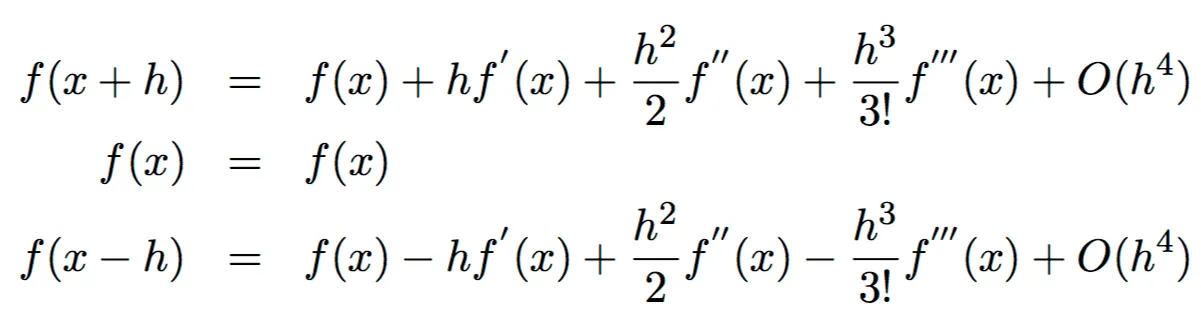
So, when the grid spacing dx (h in the above formula) is considerably a big number, then the higher order numbers can no longer be neglected. But, if the grid spacing is decreased more and more, then the truncations errors shall be negligible to affect the final solution. One way of doing this is by increasing the number of grid points. This is the rationale behind the grid independence study.
When the grid spacing is large, the truncation error is large and hence the difference of the numerical solution form the analytical solution is very large. Due to this, when we reduce the grid spacing, the numerical results change because the truncation errors have reduced and it moves closer to the actual solution. This also ensure us that our results are still influenced by the changes in the grid spacing which needs to be avoided. When we keep reducing the grid spacing to such an extent that any further reduction in 'dx' no longer changes the solution we obtain, then the solution is said to have achieved grid independence.
For our grid independence study, we take the reference of three flow variables namely density, Mach no and the velocity at the exit whose exact analytical values are 0.052, 3.359 and 1.863 respectively.
Fluid Property: Density
| No. of Grid Points(n) | Conservative | Non-Conservative |
| n=31 | 0.0526 | 0.0528 |
| n=61 | 0.0526 | 0.0526 |
| n=91 | 0.0525 | 0.0526 |
| n=121 | 0.0525 | 0.0525 |
| n=151 | 0.0525 | 0.0525 |
| n=181 | 0.0518 | 0.0525 |
| n=211 | 0.0518 | 0.0525 |
Fluid Property: Mach No.
| No. of Grid Points(n) | Conservative | Non-Conservative |
| n=31 | 3.3757 | 3.3533 |
| n=61 | 3.3629 | 3.3573 |
| n=91 | 3.3607 | 3.3582 |
| n=121 | 3.3590 | 3.3585 |
| n=151 | 3.3675 | 3.3587 |
| n=181 | 3.3537 | 3.3588 |
| n=211 | 3.3349 | 3.3590 |
Fluid Property: Velocity
| No. of Grid Points(n) | Conservative | Non-Conservative |
| n=31 | 1.8659 | 1.8618 |
| n=61 | 1.8639 | 1.8628 |
| n=91 | 1.8635 | 1.8628 |
| n=121 | 1.8633 | 1.8630 |
| n=151 | 1.8687 | 1.8630 |
| n=181 | 1.8552 | 1.8631 |
| n=211 | 1.8430 | 1.8631 |
From the above tables we see that the values of nearly all the flow variables remain the same after n=31. Increasing the number of grid point beyond this makes some minor changes in the value of density, Mach No. and velocity. Hence, we can conclude that our numerical solution achieves grid independence at n=31. But, nonetheless, we see that as we keep increasing the value of n, the solution gets more and more refined. Grid independence also depends on how much accuracy we need in our results. If our target accuracy is around 10^(-4)-10^(-5) then, we cannot claim grid independence at n=31. So, not going to too much of accuracy, we can consider that we achieve grid indepencdence at n=31.
CONCLUSION
a) From the graph that compares the steady state mass flow rate of the conservative and the non-conservative forms, we can clearly see that the conservative form provides a more accurate and stable solution of the mass flow rate than the non-conservative form.
b) From the grid independence study, we can observe that the flow properties become nearly grid independent after n=31 but upon increasing the no. of grid points we see that the stability of the values is seen more in the non-conservative form than that of the conservative form.
c) There is no clear dominance of one form of governing equations over the other. But the conclusions a) and b) clearly support the fact that the conservative form of the governing equations are more efficient in solving flux variables inside the nozzle wheares the non-conservative form provides slightly more accurate values of the primitive flow variables inside the nozzle.
d) In terms of the formulation of the problem, more effort goes in solving the nozzle problem using the conservative from the governing equation. This is because of rearranging the entire set of equation in the form of the flux variables and then extracting the values of the primitive varibles from these flux quantities. Wheares in the non-conservative from we directly solve for the primitive variables, which definitely reduces both the human effort as well as the computational effort.