Week 7 Challenge

Simulation of ID Supersonic Nozzle using Maccormack’s Technique

OBJECTIVE

In this challenge you are going to simulate the isentropic flow through a quasi 1D subsonic-supersonic nozzle. You will derive both the conservation and non-conservation forms of the governing equations and solve them using the MacCormack's technique. You need to determine the steady-state temperature distribution for the flow-field variables and investigate the difference between the two forms of governing equations by comparing their solutions.

You need to show the following plots inside your report

1. Steady-state distribution of primitive variables inside the nozzle
2. Time-wise variation of the primitive variables
3. Variation of Mass flow rate distribution inside the nozzle at different time steps during the time-marching process
4. Comparison of Normalized mass flow rate distributions of both forms

Expected Results:

• Perform a grid independence test on the solution and explain all your findings.
• The code must be modular. You need to write separate functions to solve both forms.
• Discuss all the plots you are providing with observed inferences.

Note:

Refer CFD book by John Anderson for Initial and boundary conditions.

THEORY

• Supersonic Nozzle

Nozzles are actually used to modify the flow of a fluid (i.e. by increasing kinetic energy of the flow in expense of its pressure). Convergent-divergent type of nozzles are mostly used for supersonic flows because it is impossible to create supersonic flows (Mach number more than one) in convergent type of nozzle and therefore it restricts us to a limited amount of mass flow through a particular nozzle. In convergent-divergent type of nozzles we can increase the flow velocity much higher than sonic velocity that is why these types of nozzles have a wide application such as propelling nozzles in jet engines or in air intake for engines working at high rpms. When we attach a divergent nozzle just after the convergent nozzle our flow speed starts increasing with the decrease in back pressure and also the mass flow rate. And therefore, in this type of nozzles we can reach to the speeds above sonic i.e. supersonic.

Convergent-divergent(C-D) type of nozzles have a lot of application as a propelling nozzle in automobile and jets. Few examples of the application of convergent divergent type of nozzles in engineering are Steam turbines : In power plants, Rockets : for providing sufficient thrust to move upwards and supersonic gas turbine engine : for the air intake when air requirement of engine is high. C-D nozzles can also be seen in water supply pumps or in formula car intake system

We consider the steady, isentropic flow through a convergent-divergent nozzle.The flow at the inlet to the nozzle comes from a reservoir where the pressure and temperature are denoted by p0 , and T0 , respectively. The cross-sectional area of the reservoir is large, and hence the velocity is very small. Thus, p0 and T0 are the stagnation values, or total pressure and total temperature, respectively. The flow expands isentropically to supersonic speeds at the nozzle exit, where the exit pressure, temperature, velocity, and Mach number are denoted by Pe, ,, Ve, and Me, respectively. The flow is locally subsonic in the convergent section of the nozzle, sonic at the throat (minimum area), and supersonic at the divergent section. The sonic flow (M = 1) at the throat means that the local velocity at this location is equal to the local speed of sound. Using an asterisk to denote sonic flow values, we have at the throat V = V* = a*. Similarly, the sonic flow values of pressure and temperature are denoted by p* and T*, respectively. The area of the sonic throat is denoted by A*. We assume that at a given section, where the cross-sectional area is A, the flow properties are uniform across that section. Hence, although the area of the nozzle changes as a function of distance along the nozzle, x, and therefore in reality the flow field is two-dimensional (the flow varies in the two-dimensional xy space), we make the assumption that the flow properties vary only with x; this is tantamount to assuming uniform flow properties across any given cross section. Such flow is defined as quasi-one-dimensional flow.

• Governing equations

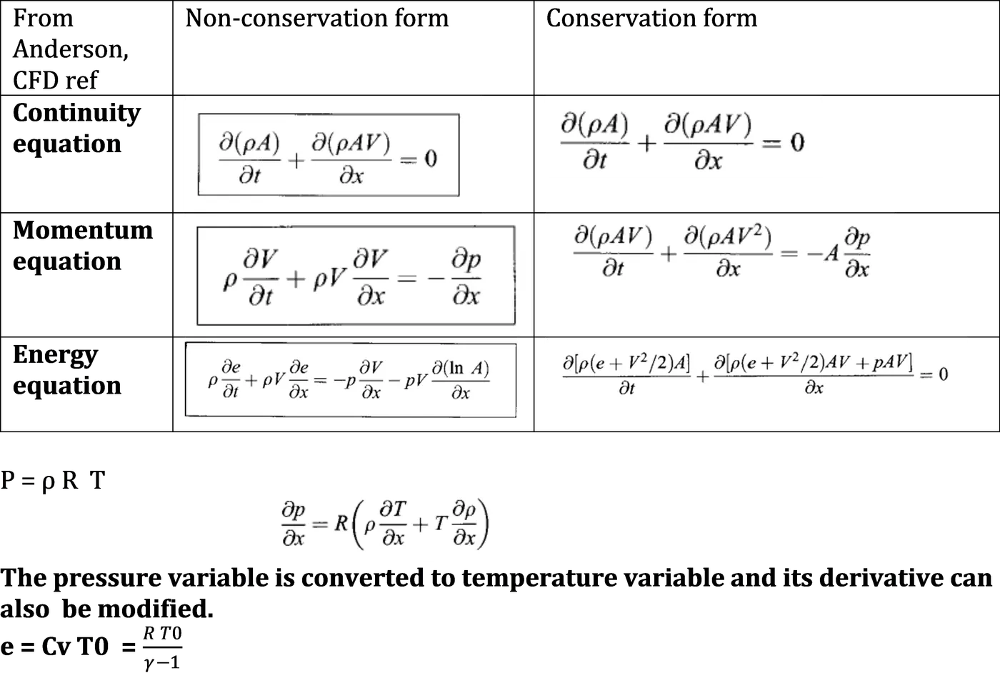
Governing partial differential equations for inviscid flow are the Euler equations for quasi one-dimensional flow

• Non- dimensionalizing of variables

Parameters are selected as dimensionless values for ρ, T and v for accurate solution.

Density (with initial density, ) `ρ’ = ρ/(ρ0)`

Temperature (with initial temperature, ) `T' = T/(T0)`

Velocity (with Mach number, `a0 = sqrt(gamma R T)` ) `v' = v/(a0)`

Distance (with length of nozzle, L) `x' =x/L`

Time (with L/a0) `t' =t/(x/L)`

Area (with area of throat, A*) `A' = A/(A**)`

Energy (with initial temperature, `e’ = e/(e0) = (Cv T)/(Cv T0) = T/(T0)`

• Non- conservation form

• Conservation form

• MacCormack’s Technique

The MacCormack's technique is a variant of the Lax-Wendroff approach but is much simpler in its application. Like the Lax-Wendroff method, the MacCormack method is also an explicit finite-difference technique which is second-order-accurate in both space and time. We assume that the flow field at each grid point is known at time t, and we proceed to calculate the flow-field variables at the same grid points at t + dt. First, consider a parameter at grid point (i, j) at time t + dt. In MacCormack's method, this is obtained from

`ρ_(i,j)^(t+dt) = ρ_(i,j)^t+ (∂ρ)/(∂x ) (av ) dt`

where derivative av is a representative mean value of derivative between times t and t + dt. The value of derivative av is calculated so as to preserve second order accuracy without the need to calculate values of the second time derivative, which is the term which involves a lot of algebra. With MacCormack's technique, this algebra is circumvented. Similar relations are written for the other flow-field variables.

Predictor step. In the continuity equation, replace the spatial derivatives on the right-hand side with forward differences. All flow variables at time t are known values. Now, obtain a predicted value of density is from the first two terms of a Taylor series. In a similar fashion, predicted values for u, v, and e can be obtained.

Corrector step. In the corrector step, we first obtain a predicted value of the time derivative at time t + dt, by substituting the predicted values of p, u, and v into the right side of the continuity equation, replacing the spatial derivatives with rearward differences. The average value of the time derivative of density is obtained from the arithmetic mean of derivative at t and derivative at t + dt. This allows us to obtain the final, "corrected" value of density at time t +dt

`ρ_(i,j)^(t+dt) = ρ_(i,j)^t+ (∂ρ)/(∂x ) (av ) dt`

The predictor-corrector sequence described above yields the value of density at grid point (i, j) at time t + dt. This sequence is repeated at all grid points to obtain the density throughout the flow field at time t + dt. To calculate u, v, and e at time t + dt the same technique is used, starting continuity equation and utilizing the momentum and energy equations to obtain the average time derivatives via the predictor-corrector sequence, using forward differences on the predictor and rearward differences on the corrector.

MacCormack's technique as described above, because a two-step predictor-corrector sequence is used with forward differences on the predictor and with rearward differences on the corrector, is a second-order-accurate method.

Stability criteria is defined by Courant number C.

`d t = C dx/ (a +v)`

METHODOLOGY

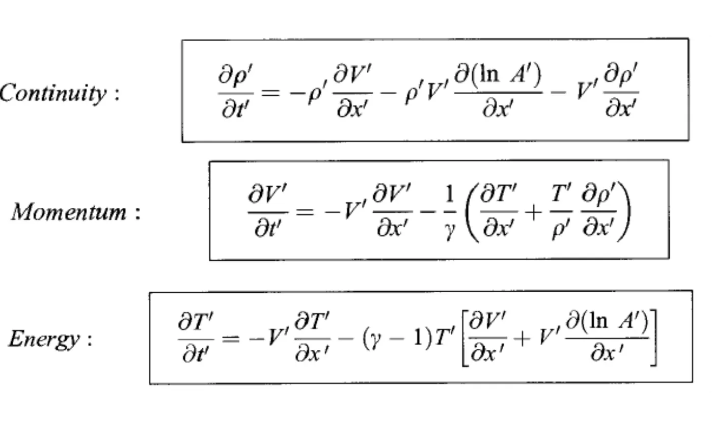
• Governing equations in non-dimensionalised Non-Conservative Form

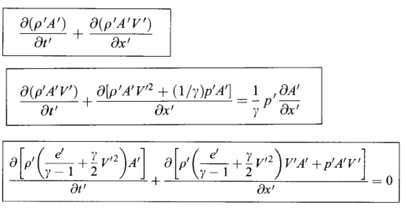
• Governing equations in non-dimensionalised Conservative Form

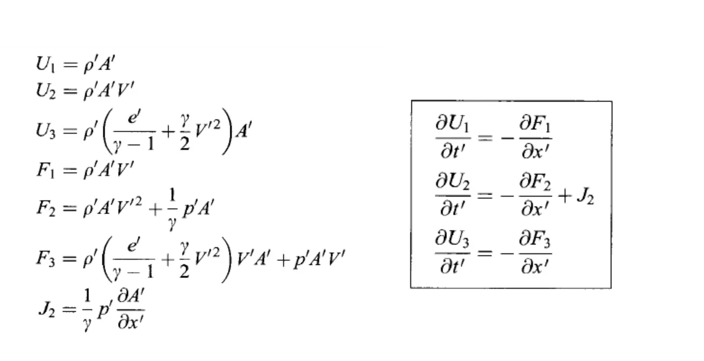
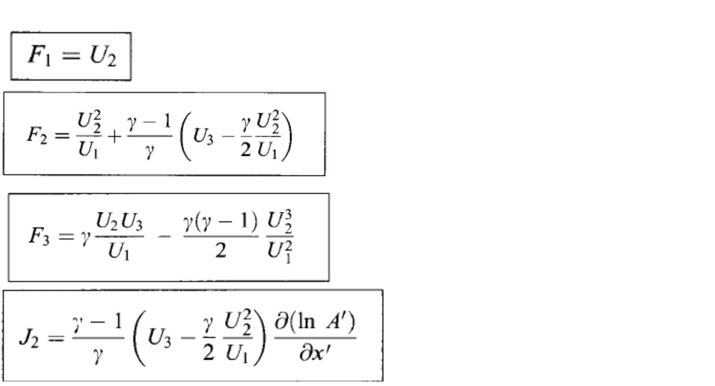
The equations for quasi-one-dimensional flow can be expressed in a similar generic form. Let us define the elements of the solutions vector U, the flux vector F, and the source term J as follows.

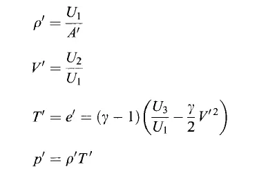
Before setting up this numerical solution, the conservation form of the equations the dependent variables (the variables for which we directly obtain numbers) are not the primitive variables. Our numerical solution will give us numbers directly for U1, U2 and U3 in steps of time; this is why u is called the solutions vector. To obtain the primitive variables (p, V, T, p, etc.), we must decode the elements U1, U2, and U3 as follows. From the definitions of U1, U2, and U3 given above, we have

CODING IN MATLAB

• Non-dimensionalised Non-Conservative Form

Solving 1D supersonic nozzle flow using MATLAB code.

Non_conservative_form.m is generated using ‘function’ command

Input parameters are selected as dimensionless values for ρ, T and v for accurate solution.

Inputs for the code are length of nozzle domain (x), dx, Number of grid points, ratio of specific heats ( ,gamma), number of iterations (nt) and Courants number (C). The outputs from the program to be stored for plotting and analysis are Mass flow rate, Pressure, Mach number, density (ρ), velocity (v), temperature (T), density at throat, velocity at throat, temperature at throat, Mass flow rate at throat, Pressure at throat and Mach number at throat.

Space discretisation

No. of grid points are chosen as 31. gamma variable is taken as 1.4. 'linspace' command is used to discretize space domain.

Time discretisation/iterations

No. of time step are taken as 2000. Courant Number is selected as 0.5 as per stability criteria.

Time-step is programmed as per the courant number criteria.

`∆t = (C ∆x)/(a + v)`

Since the Courant number is a matrix of n values the minimum value is taken for computation. C is taken as 0.5 as per Ref Anderson, CFD

Initial states

Initial states of variables and throat geometry conditions are given as per Ref. Anderson, CFD

ρ = 1 - 0.3146x

T = 1 - 0.2314x

v = (0.1 + 1.09x) T^1/2

Area & Throat profiles are provided as per the problem.

A = 1 + 2.2(x - 1.5)²

Outer Time Loop for solving the nozzle is identified with k. The initial values are stored as old values for reference and further use.

Predictor step

Time Loop for solving Predictor step is identified with j. Equation's spatial terms for , are simplified with forward differencing. Continuity Equation, Momentum Equation and Energy Equation for predictor step are written in terms of the simplified terms variable for ρ, T, v and gamma. Solution is updated with the predictor step inside the for loop.

`ρ_(Pred) = ρ_(Initial) + (∂ρ)/(∂x) (Pred)*dx`

`T (pred) = T (Initial) + (∂T)/(∂x) (pred)*dx`

`v (pred) = v (Initial) + (∂v)/(∂x) (pred)*dx`

Corrector step

Time Loop for solving Corrector step is identified with j. Equation's spatial terms for `(∂ρ)/(∂x) , (∂T)/(∂x), (∂V)/(∂x) ,(∂(log⁡a))/(∂x)` are simplified with backward differencing. Continuity Equation, Momentum Equation and Energy Equation for predictor step are written in terms of the simplified terms variable for ρ, T, v and gamma.

Final derivative

Average Time derivative for ρ, T and v with predictor step and corrector step

`(∂ρ)/(∂x) (av)= 0.5( (∂ρ)/(∂x) (pred) +(∂ρ)/(∂x) (CORRECTOR))`

`(∂T)/(∂x) (av)= 0.5( (∂T)/(∂x) (pred) + (∂T)/(∂x) (CORRECTOR))`

`(∂v)/(∂x) (av)= 0.5( (∂v)/(∂x) (pred) + (∂v)/(∂x) (CORRECTOR))`

(average)= 0.5( (predictor) (corrector))

Final Solution Update for ρ, T and v is carried out with the loop counter loop variable i

`ρ (FINAL) = ρ (Initial) + (∂ρ)/(∂x) (av)*(dt)`

Boundary Conditions

Boundary Conditions are applied at inlet and outlet using method of characteristics. At inlet

ρ = 1

v(1) = 2v(2) - v(3)

T(1) = 1

At Outlet for ρ, T and v are calculated by the formula below

ρ(n) = 2ρ (n-1) - ρ(n - 2)

T(n) = 2T (n-1) - T(n - 2)

v(n) = 2v (n-1) - v(n - 2)

We define Mass flow rate, Pressure and Mach number

Mass flow rate = ρ a v

Pressure = ρ R T

Mach number=`= v/(√(gamma R T)`

Variables at throat section is calculated to check whether choked flow is seen at the throat after sufficient iterations. Plots are generated to compare non-dimensional mass flow rates at different time steps.

• Non-dimensionalised Conservative Form

Conservative_form.m is generated using ‘function’ command

Input parameters are selected as dimensionless values for ρ, T and v for accurate solution.

Inputs for the code are length of nozzle domain (x), dx, Number of grid points, ratio of specific heats ( ,gamma), number of iterations (nt) and Courants number (C). The outputs from the program to be stored for plotting and analysis are Mass flow rate, Pressure, Mach number, density (ρ), velocity (v), temperature (T), density at throat, velocity at throat, temperature at throat, Mass flow rate at throat, Pressure at throat and Mach number at throat.

Space discretisation

No. of grid points are chosen as 31. gamma variable is taken as 1.4. 'linspace' command is used to discretize space domain.

Time discretisation/iterations

No. of time step are taken as 2000. Courant Number is selected as 0.5 as per stability criteria.

Time-step is programmed as per the courant number criteria.

`∆t = (C ∆x)/(a + v)`

Since the Courant number is a matrix of n values the minimum value is taken for computation. C is taken as 0.5 as per Ref Anderson, CFD

Initial states

Initial states of variables and throat geometry conditions are given as per Ref. Anderson, CFD

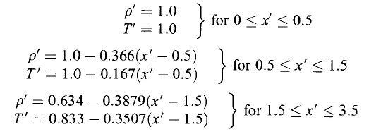
Area & Throat profiles are provided as per the problem.

A = 1 + 2.2(x - 1.5)²

Outer Time Loop for solving the nozzle is identified with k. The initial values are stored as old values for reference and further use.

Initial profile for Velocity and Pressure

`v = 0.59/(ρa)`

Pressure = ρRT

Initial Solution Vectors(U), U1, U2 and U3 are calculated

Outer Time Loop for solving the nozzle is identified with k. Time-step is programmed as per the courant number criteria

Since the Courant number is a matrix of n values the minimum value is taken for computation. The initial values are stored as old values for reference and further use. Flux vector(F) is generated for conservative form of governing equations

Predictor step

Time Loop for solving Predictor step is identified with j. Source term(J) for predictor step is calculated as ta function of gamma, density, temperature and area. Continuity Equation, Momentum Equation and energy equation for predictor step are written in simplified terms of the initial solution vectors and flux vector and source terms. Solution is updated with the predictor step inside the for loop. Flux vectors are updated with the updated solution vectors.

Corrector step

Time Loop for solving Corrector step is identified with j. Source term(J) for Corrector step is calculated as ta function of gamma, density, temperature and area. Continuity Equation, Momentum Equation and energy equation for Corrector step are written in simplified terms of the initial solution vectors and flux vector and source terms.

Final derivative

Average Time derivative with predictor step and corrector step. Final Solution Update is carried out with the loop counter loop variable i

Boundary Conditions

Boundary Conditions are applied at inlet and outlet for the solution vectors. They are specified using method of characteristics. At Inlet

U1(1) = ρ(1) X a(1)

U2(1) = 2 X U2(2) - U2(3)

v(1) = U2(1)/U1(1)

`U3(1) = U1(1) ( (T(1))/(γ - 1) + γ/(V^2) )`

At Outlet

U1(n) = 2 U1(n - 1) - U1(n - 2)

U2(n) = 2 U2(n - 1) - U2(n – 2)

U3(n) = 2 U3(n - 1) - U3(n - 2)

Finally, Primitive value updated from the solution vector.

We define Mass flow rate, Pressure and Mach number

Mass flow rate = ρ a v

Pressure = ρ R T

Mach number= `= v/(√(gamma R T)`

Variables at throat section is calculated to check whether choked flow is seen at the throat after sufficient iterations. Plots are generated to compare non-dimensional mass flow rates at different time steps.

RESULTS/PLOTS

The number of grid pints n and number of iterations are varied to find out the sensitivity.

n=31; nt = 1400

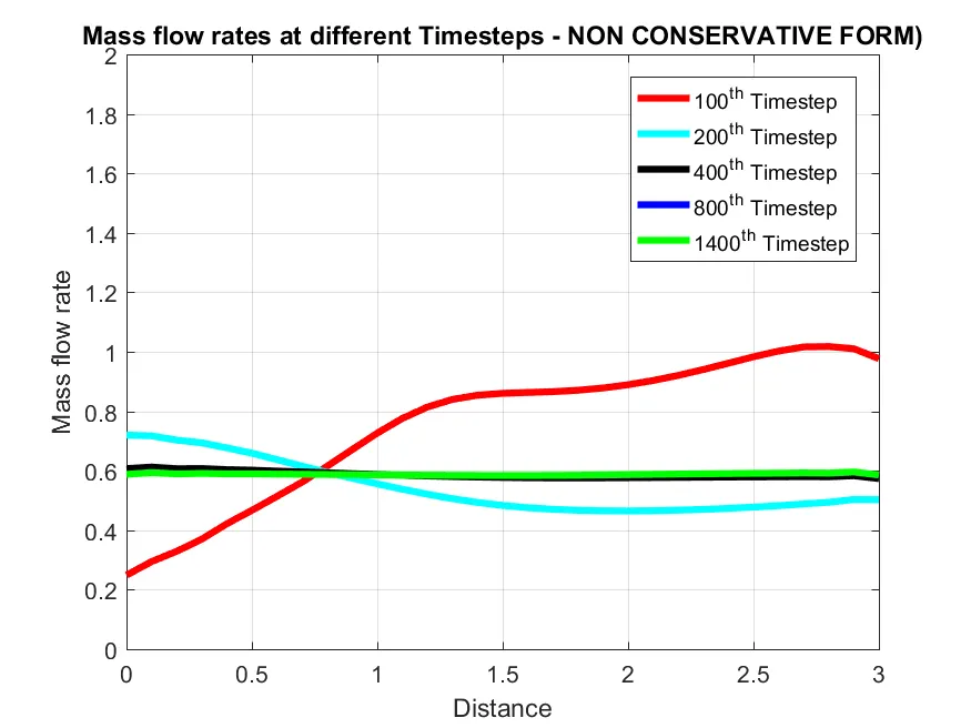
The non-dimensionalised mass flow rate at the nozzle is plotted with mass flow rate in y axis and nozzle length along x axis. We can see that a steady state mass flow rate is observed from large no. of iterations and close to the expected vaalue of 0.59.

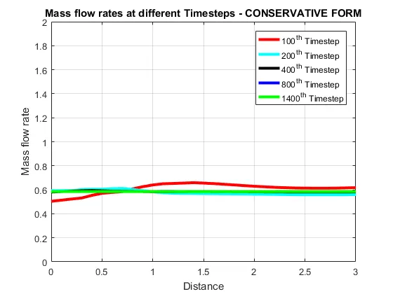
The non-dimensionalised mass flow rate at the nozzle is plotted with mass flow rate in y axis and nozzle length along x axis. We can see that a steady state mass flow rate is observed from large no. of iterations and close to the expected vaalue of 0.59. But the mass flow rate converges to steady state faster with conservative form

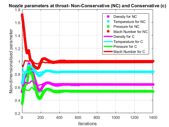
The nozzle parameters at throat is plotted with non-dimensionalised parameter along y axis and no. of iterations along x axis. The continuous line is for the numerical solution from conservative form and star is for the numerical solution from non-conservative form. The simulation results indicate that the initial errors in conservsative form is lesser than non-conservative form. But given adequate no. of iterations, both forms reach a solution.

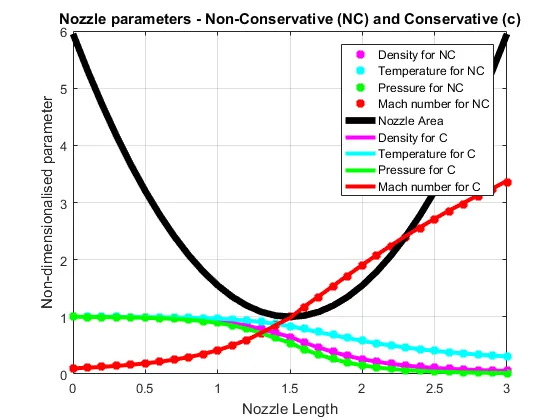
The nozzle parameters at throat is plotted with non-dimensionalised parameter along y axis and no. of nozzle length along x axis. The continuous line is for the numerical solution from conservative form and star is for the numerical solution from non-conservative form. The black line if for the non-dimensionalised nozzle area. We can see from the red line for Mach number that the Mach number is 1 at throat where non-dimensionalised area is 1. Both conservative soltion and non-conservative solutions are exactly one over other in the plot.

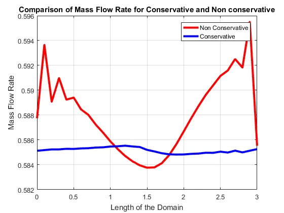
The non-dimensionalised mass flow rate is compared for Conservative form and non-conservative form for the final iteration. It can be seen that the numerical solution from conservative form is slightly more accurate in the 3rd decimal.

Grid independence

Grid independence studies are carried with n=61; nt = 1400.

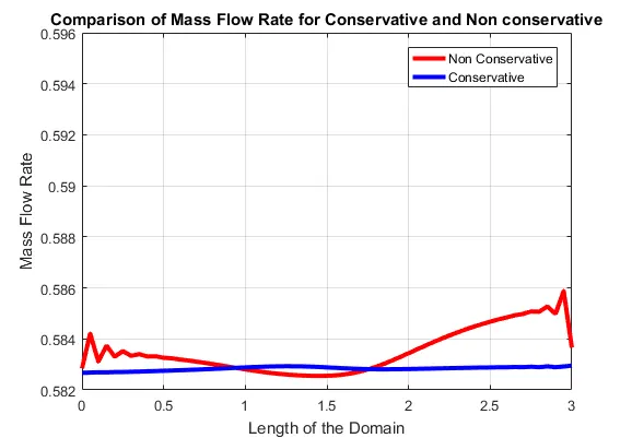
All inferences from simulation and results are similar to the case with 31 grid points. The non-dimensionalised mass flow rate comparison is plotted for conservative for mand non-conservative form. The simulation result indicate that the result is marginally improved only by increasing the grid points .hence it can be said that the solution is grid independent at 31 and 61 grid points.

CONCLUSIONS

1. 1D supersonic nozzle is simulated with MacCormack’s technique with conservative form and non-conservative form of Euler equations
2. The time taken for simulating 1D supersonic nozzle with MacCormack’s technique using MATLAB is less for non-conservative form.

	The form of governing equation	n	Iterations	Simulation time (s) *
1	Non- Conservative form	31	1400	0.0360
2	Conservative form	31	1400	0.0456
3	Non- Conservative form	61	1400	0.0475
4	Conservative form	61	1400	0.0581
5	Non- Conservative form	61	2800	0.0505
6	Conservative form	61	2800	0.0632

*Plotting time is not included in simulation time.

3. Accuracy of obtaining a steady state mass flow rate in the nozzle after 1400 /2800 iterations is checked for both forms. Accuracy is better with conservative form.
4. Grid independence is established with n= 31 and n = 61
5. Time domain independence is established with nt= 1400 and nt = 2800

PORGRAMS

Supersonic_nozzle.m

clear all;
close all;
clc;
 
%Solving 1D supersonic nozzle flow using MATLAB code. 
%Input parameters are selected for accurate solution. No. of grid points
%are chosen as 31. gamma varialbe is taken as 1.4. 'linspace' command is used to discretize space domain.
%No. of time step are taken as 2000. %Courant Number is selected as 0.5 as per stability criteria
n = 61;
gamma = 1.4;
x = linspace(0,3,n);
dx = x(2) - x(1);
a = 1 + 2.2*(x - 1.5).^2;
throat = find(a==1);
nt = 2800;
C = 0.5;
 
%FUNCTION FOR NON CONSERVATIVE FORM
tic;
[Mass_flow_rate_NC, Pressure_NC, Mach_number_NC, rho_NC, v_NC, T_NC, rho_throat_NC, v_throat_NC, T_throat_NC, Mass_flow_rate_throat_NC, Pressure_throat_NC, Mach_number_throat_NC] = Non_conservative_form(x, dx, n, gamma, nt, C);
Time_elapsed_NC = toc;
fprintf('Simulation time for Non Conservative form: %0.4f', Time_elapsed_NC);
hold on;
 
%FUNCTION FOR CONSERVATIVE FORM
tic;
[Mass_flow_rate_C, Pressure_C, Mach_number_C, rho_C, v_C, T_C, rho_throat_C, v_throat_C, T_throat_C, Mass_flow_rate_throat_C, Pressure_throat_C, Mach_number_throat_C] = Conservative_form(x, dx, n, gamma, nt, C);
Time_elasped_C = toc;
fprintf('Simulation time for Conservative form: %0.4f', Time_elasped_C);
 
%PLOTTING
%Timestep variation of properties at throat area in Non Conservative form AND Conservative form
figure(3)
plot(rho_throat_NC,'*','color','m','linewidth',3); hold on; 
plot(T_throat_NC,'*','color','c','linewidth',3); 
plot(Pressure_throat_NC,'*','color','g','linewidth',3);  
plot(Mach_number_throat_NC,'*','color','r','linewidth',3);  
plot(rho_throat_C,'color','m','linewidth',3); hold on; 
plot(T_throat_C,'color','c','linewidth',3); 
plot(Pressure_throat_C,'color','g','linewidth',3);  
plot(Mach_number_throat_C,'color','r','linewidth',3);  
hold off;
xlabel('Iterations')
ylabel('Non-dimensionalised parameter')
legend({'Density for NC','Temperature for NC','Pressure for NC','Mach Number for NC','Density for C','Temperature for C','Pressure for C','Mach Number for C'});
grid on;
title('Nozzle parameters at throat- Non-Conservative (NC) and Conservative (c)')
% saveas(1,'Supersonic nozzle throat with with nt 2800 and n = 61.png');
 
%Steady state simulation for primitve values for Non Conservative form AND Conservative form  
figure(4);
plot(x,rho_NC,'*','color','m','linewidth',3); hold on; 
plot(x,T_NC,'*','color','c','linewidth',3)
plot(x,Pressure_NC,'*','color','g','linewidth',3);
plot(x,Mach_number_NC,'*','color','r','linewidth',3) 
plot(x,a,'color','k','linewidth',5),
plot(x,rho_C,'color','m','linewidth',3); hold on; 
plot(x,T_C,'color','c','linewidth',3)
plot(x,Pressure_C,'color','g','linewidth',3);
plot(x,Mach_number_C,'color','r','linewidth',3) 
xlabel('Nozzle Length') 
ylabel('Non-dimensionalised parameter');
legend({'Density for NC','Temperature for NC','Pressure for NC','Mach number for NC','Nozzle Area','Density for C','Temperature for C','Pressure for C', 'Mach number for C'}); 
grid on;
title('Nozzle parameters - Non-Conservative (NC) and Conservative (c)')
% saveas(1,'Supersonic nozzle with nt 2800 and n = 61.png');
 
% %COMPARISON PLOT of Normalized Mass Flow Rate of both forms 
figure(5)
plot(x,Mass_flow_rate_NC,'r','linewidth',3);
hold on;
plot(x,Mass_flow_rate_C,'b','linewidth',3);
hold on; grid on;
legend('Non Conservative','Conservative');
xlabel('Length of the Domain')
ylabel('Mass Flow Rate')
axis([0 3 0.582 0.596])
title('Comparison of Mass Flow Rate for Conservative and Non conservative')
% saveas(1,'Supersonic nozzle mass flow rate with nt 2800 and n = 61.png');

Non_conservative_form.m

function [Mass_flow_rate_NC, Pressure_NC, Mach_number_NC, rho_NC, v_NC, T_NC, rho_throat_NC, v_throat_NC, T_throat_NC, Mass_flow_rate_throat_NC, Pressure_throat_NC, Mach_number_throat_NC] = Non_conservative_form(x, dx, n, gamma, nt, C)
%Function for Non-Conservative form.  Input parameters are selected as dimensionless values for ?, T and v for accurate solution. Inputs for the code are length of nozzle domain (x), dx, Number of grid points, ratio of specific heats (? ,gamma), number of iterations (nt) and Courants number (C). The outputs from the program to be stored for plotting and analysis are Mass flow rate, Pressure, Mach number, density (?), velocity (v), temperature (T), density at throat, velocity at throat, temperature at throat, Mass flow rate at throat, Pressure at throat and Mach number at throat. 
%Intial boundary conditions are given as per Ref. Anderson
rho_NC = 1 - 0.3146*x;
T_NC = 1 - 0.2314*x;
v_NC = (0.1 + 1.09*x).*T_NC.^0.5;
 
%Area & Throat profiles are provided as per the problem
a = 1 + 2.2*(x - 1.5).^2;
throat = find(a==1);
 
%Outer Time Loop for solving the nozzle is identified with k
for k = 1:nt
 
%Time-step is programmed as per the courant number criteria
dt = min(C.*dx./(sqrt(T_NC) + v_NC));
 
%The intital values are stored as old values for reference and further use. 
rho_old = rho_NC;
T_old = T_NC;
v_old = v_NC;
 
%Time Loop for solving Predictor step is identified with j.
for j = 2:n-1
 
%Equation's spatial terms for ??/?x , ?T/?x ?V/?x (?(loga))/?x are simplified with forward differencing.  
dv_dx = (v_NC(j + 1) - v_NC(j))/dx; 
drho_dx = (rho_NC(j + 1) - rho_NC(j))/dx; 
dT_dx = (T_NC(j + 1) - T_NC(j))/dx;
dlog_a_dx = (log(a(j + 1)) - log(a(j)))/dx;
 
%Continuity Equation for predictor step are written in terms of the simplified terms
drho_dt_P(j) = -rho_NC(j)*dv_dx - rho_NC(j)*v_NC(j)*dlog_a_dx - v_NC(j)*drho_dx;
 
%Momentum Equation for predictor step are written in terms of the simplified terms
dv_dt_P(j) = -v_NC(j)*dv_dx - (1/gamma)*(dT_dx + (T_NC(j)*drho_dx/rho_NC(j)));
 
%Energy Equation for predictor step are written in terms of the simplified terms
dT_dt_P(j) = -v_NC(j)*dT_dx - (gamma - 1)*T_NC(j)*(dv_dx + v_NC(j)*dlog_a_dx);
 
%Solution is updated with the predictor step inside the for loop
rho_NC(j) = rho_NC(j) + drho_dt_P(j)*dt; 
v_NC(j) = v_NC(j) + dv_dt_P(j)*dt; 
T_NC(j) = T_NC(j) + dT_dt_P(j)*dt;
end
 
% Time Loop for solving Corrector step is identified with j.
for j = 2:n-1
 
%Equation's spatial terms are simplifyed with backward differencing. 
dv_dx = (v_NC(j) - v_NC(j - 1))/dx; 
drho_dx = (rho_NC(j) - rho_NC(j - 1))/dx; 
dT_dx = (T_NC(j) - T_NC(j - 1))/dx;
dlog_a_dx = (log(a(j)) - log(a(j - 1)))/dx;
 
%%Continuity Equation for Corrector step are written in terms of the simplified terms
drho_dt_C(j) = - rho_NC(j)*dv_dx - rho_NC(j)*v_NC(j)*dlog_a_dx - v_NC(j)*drho_dx;
 
%Momentum Equation for Corrector step are written in terms of the simplified terms
dv_dt_C(j) = - v_NC(j)*dv_dx - (1/gamma)*(dT_dx + (T_NC(j)*drho_dx/rho_NC(j)));
 
%Energy Equation for Corrector step are written in terms of the simplified terms
dT_dt_C(j) = - v_NC(j)*dT_dx - (gamma - 1)*T_NC(j)*(dv_dx + v_NC(j)*dlog_a_dx);
end
 
%Average Time derivative with predictor step and corrector step
drho_dt = 0.5.*(drho_dt_P + drho_dt_C);
dv_dt = 0.5.*(dv_dt_P + dv_dt_C);
dT_dt = 0.5.*(dT_dt_P + dT_dt_C);
 
%Final Solution Update is carried out with the loop counter loop variable i
for i = 2:n-1
rho_NC(i) = rho_old(i) + drho_dt(i)*dt; 
v_NC(i) = v_old(i) + dv_dt(i)*dt;
T_NC(i) = T_old(i) + dT_dt(i)*dt;
end
 
%Boundary Conditions are applied at inlet and outlet 
%At Inlet 
rho_NC(1) = 1;
v_NC(1) = 2*v_NC(2) - v_NC(3); 
T_NC(1) = 1;
%At Outlet
rho_NC(n) = 2*rho_NC(n-1) - rho_NC(n - 2); 
v_NC(n) = 2*v_NC(n - 1) - v_NC(n - 2); 
T_NC(n) = 2*T_NC(n - 1) - T_NC(n - 2);
 
%Defining Mass flow rate, Pressure and Mach number
Mass_flow_rate_NC = rho_NC.*a.*v_NC; 
Pressure_NC = rho_NC.*T_NC; 
Mach_number_NC = (v_NC./sqrt(T_NC));
 
%Calculating Variables at throat section 
rho_throat_NC(k) = rho_NC(throat); 
T_throat_NC(k) = T_NC(throat); 
v_throat_NC(k) = v_NC(throat);
Mass_flow_rate_throat_NC(k) = Mass_flow_rate_NC(throat); 
Pressure_throat_NC(k) = Pressure_NC(throat); 
Mach_number_throat_NC(k) = Mach_number_NC(throat);
 
%PLOTTING
%Comparison of non-dimensional Mass flow rates at different time steps 
figure(1);
if k == 100
plot(x, Mass_flow_rate_NC, 'r', 'linewidth', 3);
hold on; 
elseif k == 200
plot(x, Mass_flow_rate_NC, 'c', 'linewidth', 3);
hold on;
elseif k == 400
plot(x, Mass_flow_rate_NC, 'k', 'linewidth', 3);
hold on 
elseif k == 800
plot(x, Mass_flow_rate_NC, 'b', 'linewidth', 3);
hold on 
elseif k == 1400
plot(x, Mass_flow_rate_NC, 'g', 'linewidth', 3);
hold on
end
title('Mass flow rates at different Timesteps - NON CONSERVATIVE FORM)')
xlabel('Distance')
ylabel('Mass flow rate')
legend({'100^t^h Timestep','200^t^h Timestep','400^t^h Timestep','800^t^h Timestep','1400^t^h Timestep'})
axis([0 3 0 2])
grid on
end
% saveas(1,'Supersonic nozzle with non-conservative form nt 2800 and n= 61.png');
end

Conservative_form.m

function [Mass_flow_rate_C, Pressure_C, Mach_number_C,  rho_C, v_C, T_C, rho_throat_C, v_throat_C, T_throat_C, Mass_flow_rate_throat_C, Pressure_throat_C, Mach_number_throat_C] = Conservative_form(x, dx, n, gamma, nt, C)
%Function for Conservative form.  Input parameters are selected as dimensionless values for ?, T and v for accurate solution. Inputs for the code are length of nozzle domain (x), dx, Number of grid points, ratio of specific heats (? ,gamma), number of iterations (nt) and Courants number (C). The outputs from the program to be stored for plotting and analysis are Mass flow rate, Pressure, Mach number, density (?), velocity (v), temperature (T), density at throat, velocity at throat, temperature at throat, Mass flow rate at throat, Pressure at throat and Mach number at throat. 
%Intial boundary conditions are given as per Ref. Anderson
%Determining Initial profile of Density and Temperature 
for i = 1:n
if     (x(i) >= 0 && x(i) <= 0.5)
rho_C(i) = 1; 
T_C(i) = 1;
elseif (x(i) >= 0.5 && x(i) <= 1.5) 
    rho_C(i) = 1 - 0.366*(x(i) - 0.5); 
    T_C(i) = 1 - 0.167*(x(i) - 0.5);
elseif (x(i) >= 1.5 && x(i) <= 3)
rho_C(i) = 0.634 - 0.3879*(x(i) - 1.5); 
T_C(i) = 0.833 - 0.3507*(x(i) - 1.5);
end
end
 
%Area & Throat profiles are provided as per the problem
a = 1 + 2.2*(x - 1.5).^2;
throat = find(a==1);
 
%Initial profile for Velocity and Pressure 
v_C = 0.59./(rho_C.*a);
Pressure_C = rho_C.*T_C;
 
%Initial Solution Vectors(U) , U1, U2 and U3 are calculated 
U1 = rho_C.*a;
U2 = rho_C.*a.*v_C;
U3 = rho_C.*a.*(T_C./(gamma - 1)) + ((gamma/2).*v_C.^2);
 
%Outer Time Loop for solving the nozzle is identified with k
for k =1:nt
 
%Time-step is programmed as per the courant number criteria
dt = min(C.*dx./(sqrt(T_C) + v_C));
 
%The intital values are stored as old values for reference and further use. 
U1_old = U1; 
U2_old = U2; 
U3_old = U3;
 
%Flux vector(F) is generated for conservative form of governong equations
F1 = U2;
F2 = ((U2.^2)./U1) + ((gamma - 1)/gamma)*(U3 - (gamma/2)*((U2.^2)./U1)); 
F3 = ((gamma*U2.*U3)./U1) - (gamma*(gamma - 1)*((U2.^3)./(2*U1.^2)));
 
%Time Loop for solving Predictor step is identified with j.
for j = 2:n-1
 
% Source term(J) for predictor step is calculated as ta function of gamma % ,density , % temperature and area
J2(j) = (1/gamma)*rho_C(j)*T_C(j)*((a(j + 1) - a(j))/dx);
 
%Continuity Equation, Momentum Equation and energy equation for predictor step are written in simplified terms of the iniial solution vectoes and flux vector and source terms
dU1_dt_P(j) = -((F1(j + 1) - F1(j))/dx);
dU2_dt_P(j) = -((F2(j + 1) - F2(j))/dx) + J2(j);
dU3_dt_P(j) = -((F3(j + 1) - F3(j))/dx);
 
%Solution is updated with the predictor step inside the for loop
U1(j) = U1(j) + dU1_dt_P(j)*dt; 
U2(j) = U2(j) + dU2_dt_P(j)*dt; 
U3(j) = U3(j) + dU3_dt_P(j)*dt;
end
 
%Flux vectors are updated with the updated solution vectors
F1 = U2;
F2 = ((U2.^2)./U1) + ((gamma - 1)/gamma)*(U3 - ((gamma*0.5*(U2.^2))./(U1)));
F3 = ((gamma*U2.*U3)./U1) - ((gamma*0.5*(gamma - 1)*(U2.^3))./(U1.^2));                                                                    
 
% Time Loop for solving Corrector step is identified with j.
for j = 2:n-1
 
% Source term(J) for Corrector step is calculated as ta function of gamma % ,density , % temperature and area
J2(j) = (1/gamma)*rho_C(j)*T_C(j)*((a(j) - a(j - 1))/dx);
 
%Continuity Equation, Momentum Equation and energy equation for Corrector step are written in simplified terms of the iniial solution vectoes and flux vector and source terms
dU1_dt_C(j) = -((F1(j) - F1(j - 1))/dx); 
dU2_dt_C(j) = -((F2(j) - F2(j - 1))/dx) + J2(j); 
dU3_dt_C(j) = -((F3(j) - F3(j - 1))/dx);
end
 
%Average Time derivative with predictor step and corrector step
dU1_dt = 0.5*(dU1_dt_P + dU1_dt_C); 
dU2_dt = 0.5*(dU2_dt_P + dU2_dt_C); 
dU3_dt = 0.5*(dU3_dt_P + dU3_dt_C);
 
%Final Solution Update is carried out with the loop counter loop variable i
for i = 2:n-1
U1(i) = U1_old(i) + dU1_dt(i)*dt; 
U2(i) = U2_old(i) + dU2_dt(i)*dt; 
U3(i) = U3_old(i) + dU3_dt(i)*dt;
end
 
%Boundary Conditions are applied at inlet and outlet 
%At Inlet
U1(1) = rho_C(1)*a(1); 
U2(1) = 2*U2(2) - U2(3);
v_C(1) = U2(1)./U1(1);
U3(1) = U1(1)*((T_C(1)/(gamma - 1)) + ((gamma/2)*(v_C(1)).^2));
%At Outlet
U1(n) = 2*U1(n - 1) - U1(n - 2); 
U2(n) = 2*U2(n - 1) - U2(n - 2); 
U3(n) = 2*U3(n - 1) - U3(n - 2);
 
%Finally Primitive value updated from the solution vector
rho_C = U1./a;
v_C = U2./U1;
T_C = (gamma - 1)*((U3./U1 - (gamma/2)*(v_C).^2));
 
%Defining Mass flow rate, Pressure and Mach number
Mass_flow_rate_C = rho_C.*a.*v_C; 
Pressure_C = rho_C.*T_C; 
Mach_number_C = (v_C./sqrt(T_C));
 
%Calculating Variables at throat section 
rho_throat_C(k) = rho_C(throat); 
T_throat_C(k) = T_C(throat); 
v_throat_C(k) = v_C(throat);
Mass_flow_rate_throat_C(k) = Mass_flow_rate_C(throat); 
Pressure_throat_C(k) = Pressure_C(throat); 
Mach_number_throat_C(k) = Mach_number_C(throat);
 
%PLOTTING
%Comparison of non-dimensional Mass flow rates at different time steps 
figure(2)
if k == 100
plot(x, Mass_flow_rate_C, 'r', 'linewidth',3);
hold on 
elseif k == 200
plot(x, Mass_flow_rate_C, 'c', 'linewidth',3);
hold on 
elseif k == 400
plot(x, Mass_flow_rate_C, 'k', 'linewidth',3);
hold on 
elseif k == 800
plot(x, Mass_flow_rate_C, 'b', 'linewidth',3);
hold on 
elseif k == 1400
plot(x, Mass_flow_rate_C, 'g', 'linewidth',3);
hold on
end
title('Mass flow rates at different Timesteps - CONSERVATIVE FORM')
xlabel('Distance')
ylabel('Mass flow rate')
legend({'100^t^h Timestep','200^t^h Timestep','400^t^h Timestep','800^t^h Timestep','1400^t^h Timestep'})
axis([0 3 0 2])
grid on
end
% saveas(1,'Supersonic nozzle with conservative form nt 2800 and n = 61.png');
end